I have written earlier on the analysis of a 2D rotating frame, and accelerating on a swing (which is a 2D rotating frame with a constant gravitational force). Here I continue this effort to present a model of 3D rotation from which the gyroscopic effect can be obtained. The model developed here is for a point mass on a string connected to a fixed origin, with forces acting on the mass in three orthogonal directions depending on its position and velocity. The conclusions from this model can be extrapolated to solid rotating objects, or used directly to elucidate the arts and sports which involve spinning objects attached to a rope. A mathematical treatment of a disc gyroscope motion under constant precession is presented later, and some differences between these two approaches are discussed.
When swinging a mass on a string in one's hand, such as in glowsticking or fire spinning, one controls the trajectory of the mass in space by moving the hand (which is the origin point for this system) and thus changing the direction in which the string pulls the mass. There are three such orthogonal motions possible: first involving the radius, second involving the forward velocity, and third involving the transverse velocity. Note that, unlike the constant fixed X,Y,Z axes of Euclidean space, the basis of the 3D rotating system within Euclidean space constantly changes for a moving mass. The radial force is in the direction of the string, the forward force is in the direction of the forward velocity (less radial velocity), and the transverse force is perpendicular to the previous two directions. At zero velocity or zero radius, this basis is not well defined. For the performer holding the end of the string, the representation of the spherical basis forces is more useful. Indeed I would argue that a practical understanding of the gyroscopic effect in this system is essential to mastery of the spinning art.
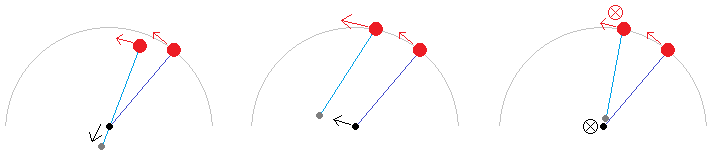
Left to right, an illustration of three orthogonal motions that a person holding a swinging mass on a string could perform: radial, forward, and transverse (in / out of the page).
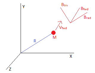
An illustration comparing a static Euclidean frame (X,Y,Z) where the axes are fixed in space while the mass moves on a string around the origin, and a rotational basis linked to the mass (B_rad,B_fwd,B_trv) which rotates in the Euclidean frame as the mass moves. These are the directions of radial force, forward velocity, and transverse direction which is perpendicular to the previous two.
Transverse acceleration is a rather strange thing, because its direction is defined as being always perpendicular to the direction of forward velocity, so as soon as it effects a slight increase of velocity in its acting direction, this direction changes so it is no longer aligned with the new velocity (therefore transverse acceleration cannot do physical work). Radial acceleration (at constant radius) is of the same nature, and in a 2D plane the radial acceleration of centripetal force maintains a constant velocity magnitude while rotating the direction of the velocity vector so the object travels in a circular path. Considering a mass on a string traveling in a circle about the origin, which is a 2D plane, adding on a transverse acceleration will deviate the motion out of this plane by rotating the velocity vector out of the circle in the direction of the circle normal vector. Note that in a real gyroscope or gimbal mount, tilting the gyroscope does not necessarily equate to transverse acceleration, because the basis is dependent on the velocity of the points on the disk (for instance with a stationary gyroscope, tilting it would be a forward acceleration, which can do physical work).
To visualize this, I wrote a Scilab script that uses a simple second-order numerical integration (velocity Verlet type) to apply forces on the rotational basis which is constantly updated for the latest position of the mass. In fact because of symplectic conservation with position if applying second order equations of motion (as also with the leapfrog algorithm), the radius of the mass is effectively kept constant by an accurate centripetal force expression (that is, without forcing the radius to be constant numerically). The velocity, however, is sensitive to the time interval between iterations, because that expression is not second order (as it combines multiple rotations of the velocity vector but in a linear manner), and with coarse time steps will tend to increase in magnitude over time. Conversely, finding that at the end of iterations the velocity magnitude has not changed much is an indicator that the simulation time steps are adequately short.
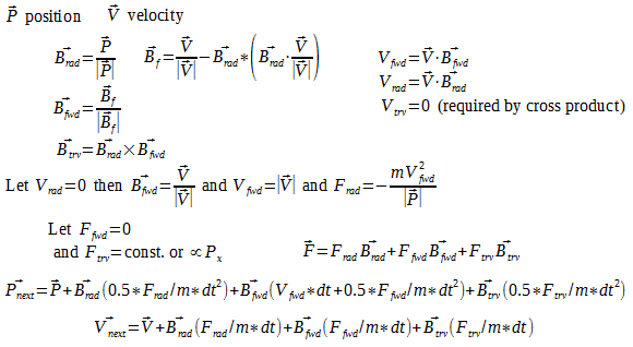
An overview of the formulas used in the simulation to calculate the spherical basis and iterate position and velocity of the mass. (Note that the code has a few additional calculations and simplifications that are not displayed here.)
What happens with a constant transverse acceleration applied to a moving mass on a string? At first I thought there would be complicated figure-8 shapes and spirals, but in actuality, the model shows that the mass will be accelerated to some limiting forward velocity magnitude at which point its trajectory will approach a circle in a static plane offset from the origin, with the offset increasing at higher transverse acceleration. This is in fact what we can observe when holding a string with a mass at the end, and then swinging the mass in a circle parallel to the ground: the downward pull of gravity can be decomposed into an increased radial force which is countered by the string and hand thus making no contribution to the trajectory, and a constant transverse force which maintains the circular trajectory in a plane offset from the sphere origin (the hand holding the string). In the absence of gravity (and other transverse forces) such a trajectory would not be stable, instead the trajectory would become a full circle about the origin at the same (linear) velocity.
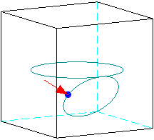
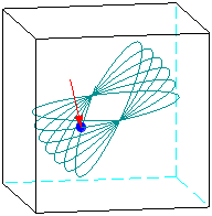
One frame of the constant transverse force simulation. The smaller circle is traversed with the constant transverse force, while the larger circle is under zero transverse force. The mass is virtually held on a string about the origin. The red arrow shows the direction and magnitude of transverse force; forward force is zero and radial force is not shown.

Animated image of the simulation of a constant transverse force applied for one revolution. The red arrow shows the direction and magnitude of transverse force; forward force is zero and radial force is not shown. These differ by 3 degrees and may be viewed in 3D by overlapping the two images with the eyes (parallel viewing).
More interesting behavior arises when the transverse acceleration is not constant but rather a function of position on the sphere. This is the case with a torque applied to a spinning gyroscope - there will be areas on the sphere where the effective force or displacement from the torque is highest, and other areas where it is lowest. It might not be obvious that the gyroscopic effect applies not only to spinning disks and solid objects but also to a point mass on a string - the effect may be confirmed experimentally by swinging an object on a string and attempting to change its plane of rotation. A solid disk may be viewed as a number of point masses, with additional forces locking them together in a rigid structure so their paths are slightly different, though the distinction becomes less critical at high rotational rate relative to precession (this may be confirmed in the formulas below).
With a gyroscope, applying a torque to turn the spin axis causes the transverse force to be a function of the distance from the plane formed by the spin and torque axes. In the point mass simulation, this is coded by making the transverse force proportional to the X coordinate of position, and the result is the rotation of the orbit about the X axis. The same counterintuitive feature as in the gyroscope is observed, since the point of highest transverse force (the pole of the sphere at maximum or minimum X coordinate) achieves net zero displacement (the mass continually passes through this point), while the point of zero transverse force (the equator of the sphere in YZ plane at X=0) achieves the highest displacement (the mass passes through a different point on the equator in each orbit). This is illustrated in the animation below.
One frame of the position-dependent axially symmetric transverse force simulation.

Animated image of the simulation of a position-dependent transverse force applied for six revolutions. The left and right views differ by 3 degrees and may be seen in 3D by overlapping the two images with the eyes (parallel viewing).
As the mass travels faster, adjacent orbits get increasingly closer together, and the behavior is qualitatively same as shown above which matches the presentation in physics lectures, where to simplify the math it is assumed that rotation angular velocity is much faster than precession angular velocity. With the numerical model, we have the ability to see what happens when this is not the case. As we slow down the mass velocity, the orbits become decidedly non-circular but they still pass through the poles (of maximum transverse force) and in between the poles they shift by a constant amount about the axis of symmetry from one orbit to the next. This is illustrated below.
Animated image of the simulation of a position-dependent transverse force applied with a slow velocity.
The particular nature of the function relating X coordinate (say) to transverse force does not matter - the same qualitative features are observed if it is linear (as used above), quadratic, or square-root; the main requirement is that the transverse field is radially symmetric about some axis (X in this case) and having a maximum at one pole (+X), while being of the opposite sign on the other side (-X) of an equator plane perpendicular to the symmetry axis (YZ). Note that while the above simulations had the initial conditions configured so the mass would travel through stationary points at the "north and south poles", it is not always the case that the mass must pass through such points. These will only exist if the mass is on a trajectory that passes through one of the poles (points of maximum transverse acceleration in a symmetric transverse acceleration field), in which case it will necessarily return to that pole repeatedly, and if it also passes through the equator, then it will necessarily visit the opposite pole before returning to the starting pole. If the mass is not on such a trajectory, then it moves in a shifting path that never reaches the poles so there are no stationary points. This is illustrated below with the velocity at the equator being such that the transverse force field deviates the path from reaching the pole before returning back to the equator.
Animated image of the simulation of a position-dependent transverse force with the mass not reaching the poles.
You may envision that as the velocity becomes increasingly slower, with the transverse force field as defined above, at some point the mass starting at a pole will be unable to cross the equator, as it will be accelerated transversely back to its starting pole. This is indeed the case (not illustrated here as it's not too informative). However, at a velocity that is just barely enough to cross the equator, an interesting trajectory is seen - one that starts at a pole, then is accelerated transversely to loop around a few times near the equator, almost traveling parallel to the equator, and subsequently crossing the equator and performing the same motions in the reverse sense to end at the opposite pole. There would be some exact initial velocity with which the mass could start at the pole and end orbiting on the equator indefinitely (an unstable equilibrium); above this velocity the mass will reach the other pole and below this velocity the mass will return to its starting pole, and the closer to this velocity, the more loops adjacent to the equator will be part of the trajectory.
Animated image of the simulation of a position-dependent transverse force applied with a very slow velocity. Note that the view presented here is rotated relative to above so that the symmetry axis is more visible.
The above numerical model confirms that a point mass influenced by position-dependent transverse acceleration in a 3D rotational frame takes on the behavior of a gyroscope, namely rotating its orbit about a perpendicular axis to the applied torque. It would be instructive to compare this to the motion of a rigid disc in a gyroscope. A different approach is taken here: we define the spin angular velocity ω and the precession angular velocity ψ, then calculate the position, velocity, and acceleration based on the expected motion of a point on a spinning disc held in a gimbal mount. The precession is taken to be externally caused. Then, by calculating the transverse force on such a point which is required to keep a given precession rate, we will find that it matches what we intuited above - that it is proportional to distance from a plane that passes through the spin axis and the torque axis. We also find that at ω comparable to ψ, there is a nonuniform distribution of radial and forward accelerations required to maintain the path imposed by the rigid disc, which means that the disc material is strained under such motions. The calculations and simulations are done in a Scilab script which can be downloaded above (or here).
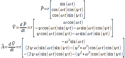
Formulas used to define the analysis. Starting from position defined by (r,ω,ψ), we obtain velocity and acceleration in 3D Euclidean space.
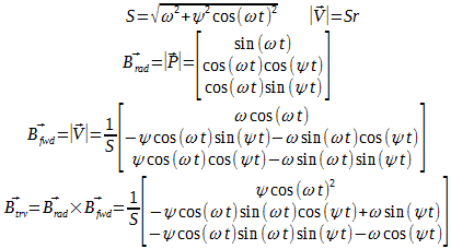
These are the definitions of a spherical basis in the Euclidean space, with the radial, forward, and transverse unit vectors.
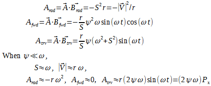
The 3D acceleration in Euclidean (static) frame is represented in the spherical rotating frame by reference to the above basis definitions. The components then are accelerations in the radial, forward, and transverse directions.
From this, we can also calculate the torque that must be applied to achieve the observed transverse acceleration. By integrating the moment contributed from each point around the orbit, with the assumption that precession is slow compared to spin (so the orbits are effectively circular), we obtain the standard expression for precession rate shown below.
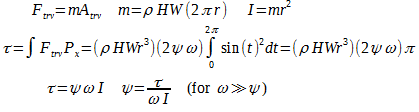
An expression relating precession rate and torque based on the above model.
We can also simulate motions where precession is similar to spin angular velocity, in which case the orbits are highly non-circular. The results here are different from the "mass on a string" model above, because here we assume the constant spin rate of a rigid disc, and to achieve this a non-uniform forward acceleration field must be present. This acceleration is done by the interatomic bonds of the rigid disc to keep a constant angular velocity (the acceleration averages out to zero over one orbit). Visually interesting shapes appear when the precession and spin rates are multiples, such as in the rendering below where the precession rate is half of the spin rate.
Animated image of the path of a point on a gyroscope disc when the precession rate is half of the spin rate. Green arrows are added to show the forward basis acceleration; note that the forward acceleration arrow is drawn 10x longer than if it were scaled to transverse acceleration, in order to make it more visible (that is, in a properly scaled image the green arrows will be 10x shorter than seen here).
Consider a stationary solid sphere centered at the origin that we want to spin up about the X axis. To do this, we would need to apply a torque about the X axis and within the YZ plane, so for instance a positive force (towards Z+) at +Y and a negative force (towards Z-) at -Y, or similar at +Z and -Z. In any case, applying the forces in the XY or XZ planes would not spin the sphere about the X axis, which is intuitively obvious. With a gyroscope, the difference is that the sphere is already spinning. Let's assume it is spinning about the Y axis. Then if we want it to spin about the X axis, we still need to accelerate it in the YZ plane (and decelerate it in the XZ plane). If we have a limitation that we can only act on the spin axis of the sphere, the need is then to apply a torque to push the spin axis from Y towards Z (in the YZ plane, simultaneously accelerating and decelerating the respective orthogonal spins) rather than from Y towards X, because moving from Y towards X would spin it about the Z axis which does not help at all. The counterintuitive part is that by pushing from Y towards Z, the spin axis actually moves towards X, but this is in the nature of how rotation is defined, made more vivid by the unusual mounting system of a gyroscope gimbal. So, holding a gyroscope on a two-bearing tilting mount in one's hand, a rapid rotation of the arm about its long axis will serve to bring the spin axis in line with this axis, just as doing this with a stationary sphere would bring its new spin axis in this line. This is the same principle used in gyrocompasses to orient the gyroscope to true north, as the rotation of the earth acts like the rotation of the arm, tending to align the spin of the gyroscope to its axis.
Animated image of gyroscopic precession as seen by an observer in the lab frame. The six blue points represent masses on the gyroscope disc, and the arrows with sphere outlines represent the lab reference frame orientation and torque applied onto the disc.
Another rather unusual interpretation is to change the reference frame so you observe the gyroscopic action from the same frame as the spinning disc; then the disc appears stationary while the world spins around it. As this happens with a torque applied to the gyroscope, the direction of torque from the external world (which is constant in the lab frame) constantly rotates and acts in different directions on the stationary disc, so that at one moment it pushes the disc one way, and a little bit later it pushes the disc the other way, and if this change in direction is fast enough relative to the torque's action on the disc's moment of inertia, then effectively the disc absorbs momentum and then returns it back to the external world without a net deviation in the process. The motion that does occur between these points is in the direction of the initial push, but by the time there is displacement of the disc in that direction, the world has rotated such that this displacement is not anymore in the direction of the applied torque, which is the gyroscopic precession. Reduced to 1D, this is like pushing a mass one way and then pushing it the other way, resulting in a transfer of force via the mass but without net travel or a direct contact between the pushing influences. The more rapidly this is done, the less displacement of the mass is necessary to transfer a large force, akin to how under a constant torque a faster spinning gyroscope will have a slower precession.
Animated image of gyroscopic precession as seen by an observer on the spinning gyroscope disc, to contrast with the lab frame rendering above. The six blue points (masses on the disc) appear stationary in this reference frame, while the surroundings and the torque applied onto the disc (red arrows) appear to rotate.
Note that the impressiveness of the gyroscopic effect relies on a particular mounting system which has low friction and high freedom of movement along orthogonal axes. By pushing on the spin axis, the axis of the gyroscope is seen to move along a perpendicular direction to the push. However if this motion is blocked by a solid bearing frame which transfers all torque (except for the push force) to the earth without deflection, then pushing the spin axis will be as easy with the gyroscope spinning as without. This is because the gyroscope actually does not present any counter-force to the push of the spin axis, hence it is not more "stable" than a non-rotating object, rather in the absence of a perpendicular force it will rotate its axis in response to the applied force. If allowed to rotate (or rather precess), then akin to the phase transition of boiling water keeping a constant temperature until all the water has changed phase, the gyroscope will not budge on the perturbation axis until its spin has aligned (to some degree) with the perturbation torque. The traditional physics class demonstration of a gyroscope on a 3-axis orthogonal gimbal keeping a stable heading is misleading in this sense, because it suggests that spinning up the gyroscope somehow increases its pointing stability. In actuality, with good enough bearings in this demonstration, the gyroscope when moved about will point in the same direction even when it is not spinning, due simply to its inertia. The spinning gyroscope does stabilize the innermost rotational axis of the mount - which is not the spin axis of the gyroscope - against one perturbation axis (that orthogonal to the spin and innermost rotational axes) and over a limited range (while the spin and perturbation axes remain orthogonal). As this single stabilized axis interacts with other bearings in the gimbal, the gimbaled gyroscope does appear more stable once spinning, but with a keen eye one will see that the spin axis regularly deviates from its starting point when the gimbal is moved about in such a demonstration.
With flying objects like frisbees, the interaction with the air is such that a constantly rotating single perturbation axis averages out to an overall zero effect, as opposed to a non-spinning frisbee where the perturbation remains in a similar direction and adds up over time: the effect of the spin is to rotate the perturbation axis, not to oppose the perturbation force or to stabilize the spin axis. So why are spinning gyroscopes used in navigation systems, instead of just stationary spheres? Their increased sensitivity to turn rate is key, for they are used as sensors (hence the "scope" suffix). One of the axes is rigidly mounted to the frame, and the torque or displacement along an orthogonal axis to the sensed one is a much-amplified output of the original rotation which can be measured locally. As in an electrical transformer, a turns ratio is achieved: the single turn of the vehicle, and the numerous turns of the gyroscope disc performed in the same time, yielding the amplification. Note that the amplification is a matter of making rotation easier to measure, as the gyroscope does not absorb or release energy during its action (the output force is at zero displacement, or the output displacement is at zero force; if there is any energy transferred it comes from the prime source of rotation and is bound by angular momentum conservation). For 3-axis stabilization, the physically amplified output of rotation from 2 or 3 gyroscopes along orthogonal axes is used in an electrically amplified feedback loop to exert an opposing force against the perturbation (which the gyroscopes by themselves cannot do).
What about the stability of the spinning top, or the ability of the spinning bicycle wheel to hang from one end of its axial rod? Once again there is an averaging effect by rotating the perturbation axis so that total perturbation remains centered on zero. Consider a 2D scenario where a reaction wheel is attached to a rigid rod. Then, the end of the rod may be supported by a string, and if the reaction wheel accelerates sufficiently to present a counter-torque against its gravitational moment, then it will be suspended in mid-air to the side of the string, like the mysterious gyroscope. Here, energy is added to the reaction wheel during acceleration, and the angular momentum of the wheel is countered by the angular momentum of the earth-wheel system through the gravitational torque. Within practical limits, this can only persist for a little bit of time, since the reaction wheel cannot accelerate indefinitely. However, if we then move the spinning reaction wheel onto the opposite side of the string, so the torque required to maintain it upright is now opposite, then we can accelerate the reaction wheel in the opposite direction (slowing down and reversing), thus holding this position for another short while on the other side. Next we can move it back, and continue repeatedly in this manner, such that the supporting string is never directly above the center of mass.

The "bicycle wheel" gyroscope demonstration is shown here schematically in 2D with a reaction wheel that accelerates in one direction, then its support is changed to the other side, allowing angular acceleration in the opposite direction for some time, then repeating the process. The red arrows signify the velocity of the reaction wheel, and the blue arrow signifies the force exerted by the accelerating wheel on to the supporting string (light blue) via a rigid rod (dark blue).
The gyroscope is the 3D extension of this, where instead of a transfer of energy from the outside as in an accelerating reaction wheel, the energy comes from the existing spin of the gyroscope, but is redirected from one rotational axis to another, in the process generating a counter-torque. Note that when the gyroscope spins 180 degrees about the string, its angular momentum in the observer frame has completely reversed. An equivalent angular momentum has been exchanged with the earth-gyroscope system due to the offset gravitational torque exerted by the suspended mass during this time, so total momentum is conserved. The precessing gyroscope (one loaded by a constant torque) is thus a stable arrangement of matter in the absence of frictional forces, that is the applied torque will not slow down or speed up the gyroscope's spin and the precession can persist indefinitely.

One frame of the very slow velocity relative to transverse acceleration simulation (animated version was presented above).
With symmetric transverse forces which increase away from the equator, as with the gyroscope, a circular trajectory is caused to rotate. As the speed of the trajectory relative to the forces is decreased, the forces will accelerate the mass from the poles to a nearly circular orbit around the equator, returning back to the poles eventually, as discussed above. If we plot this path, this may remind us of the unusual behavior of a spinning wing nut. Mentally we might visualize the "blue point" in the simulation as being attached to one of the distant points of the "wings" on the wing nut - performing a few orbits near the equator, then a flip motion where the wing tips pass near one of the poles, then a few more orbits near the equator, and a pass towards the opposite pole. (As before, the trajectory does not need to actually reach the poles and may turn back towards the equator without doing so, resulting in a "partial flip" instead of a full one.) Here the transverse force is generated internally by an imbalance in the rotation of the solid body, with the force being a function of deviation from an original axis, similar in principle to what has been coded in the simulation. Because the solid body rotates as one piece, any imbalance is constantly aligned in the rotating reference frame of the body, making a "true" transverse acceleration. It would be satisfying to prove that this is the most complex motion for a rigid body floating in space.
The Foucault Pendulum gives an impressive local measurement of the Earth's rotation. A question arises whether a gyroscopic effect is important in this 3D situation, which would be expected to be highest at the equator when the pendulum swings along the longitudinal lines. Because the pendulum swings back and forth regularly, the gyroscopic effect on one swing is canceled by a reverse gyroscopic effect on the return swing, so the observed rotation of the pendulum is not due to the gyroscopic effect (parallel transport around a spherical surface gives a better explanation). Nonetheless, the effect is real as reported in [R. Verreault's Gyroscopic theory of the Foucault pendulum: New Berry phases and sensitivity to syzygies]. (Note that parallel transport may also be applied to elucidate the gyroscopic effect following the trajectory of the point mass in the above presented model.) If a gyroscope were to be placed at the equator, then by the gyroscopic effect in an appropriate mounting it can be expected to eventually align with the earth's spin axis, which is a principle used in the gyrocompass. The applications of the gyroscope in observing earth's rotation (and the very term "gyroscope") are also credited to Foucault.
Both of the above models treated the case where a spinning gyroscope is either subject to a constant transverse torque (resulting in a constant precession angular velocity) or to a constant precession angular velocity (resulting in a constant transverse torque). The axes are orthogonal - the torque acts on zero displacement and does no work, while the displacement of precession acts on zero torque and does no work. It may then seem that there is no way to extract energy from a gyroscope or by using a gyroscope. However this analysis is particular to ω ≫ ψ, and ignores a whole range of dynamic motions when ω ≈ ψ or even ω < ψ.
A general statement will suffice to address schemes about harvesting energy from the earth's rotation (or other rotating frames): all is predicated on exchange of net angular momentum. Unless some celestial body in outer space is being accelerated or decelerated by the earth's rotation, via the device in question, there is no way to extract energy from the rotation, no matter what mechanism is used. I think the idea of using a gyroscope in this manner, such as {spinning it up at the north pole with the spin axis along the horizontal then as the earth rotates the spin axis will appear to rotate relative to the ground}, is based on an incorrect intuition of gyroscopic motion. The popular account of the gyroscope spin axis somehow being locked into absolute space, as one may be led to conclude from the physics class gimbal demonstration, is probably a driving factor, but this view is misleading as explained above. The spin axis will indeed remain constant in the absence of perturbation - but this is true for any object. Spinning up the gyroscope does not change its moment of inertia, which dictates how much the axis is accelerated by a perturbation torque, so its spin axis is not any more "locked" by the spin, rather perturbing this axis makes for some unusual motions and forces compared to the non-spinning case, and the angular acceleration is identical. If we actually set up a gyroscope at the north pole in this manner, when we start it spinning it already has angular velocity about the earth's rotation axis. As it spins up, perhaps on a single-axis gimbal, it will tilt upwards until its spin axis is aligned with the earth's rotation axis. If the upward tilt is blocked, then no energy is extracted, and if it is permitted, then the spin axis will eventually align with the rotation axis (this is not a problem because we can spin down the gyroscope, tilt it back down, and start over again). If we spin down the rotation-aligned gyroscope, the required torque is perpendicular to when we spun it up at the start, but it has its counterpart in the gyroscopic torque that was transferred to the earth as the gyroscope was tilting. During the tilt process, as the spin axis comes into alignment with the earth's rotation, energy may be extracted from the tilt motion, but this energy must come from what has previously been put into spinning up the gyroscope disc and not from the earth (note the direction of torques for the initial spin-up and extraction - they match and are perpendicular to the earth's rotation axis so total angular momentum is conserved).
As for extracting energy from the spinning disc inside the gyroscope, it is a captivating question; from the previous sentence we get an indirect sign (by angular momentum conservation) that this is possible, but how far can we go? Posed more broadly, if we have a mass attached to a shaft that is held on frictionless bearings, with these bearings held within a rigid external frame, and we can apply forces and torques only to the external frame, is it possible to change the angular velocity of the mass around the shaft? (To be precise, this velocity would be in the absolute rotational reference, so we can't just set the frame spinning about the mass and call it done.) The question is tricky, all the more so because any mechanical model will have real bearings with friction likely varying with applied torque, and any numerical model will be subject to various errors which may give an apparent small velocity or acceleration when the real answer should be zero. Thus the question can only be answered through mathematical and physical logic, and I would invite the interested reader to formulate his own answer before proceeding to the next paragraph.
Strangely enough (or perhaps just as strange as may be expected given the topic) the answer is in the affirmative. This is not strictly about the gyroscopic effect, but more about the way one may interact with a mass on frictionless bearings. We can progress from the more basic to the more exotic cases in the answer. For clarity I will define "spin axis" as that axis which is held on frictionless bearings and cannot be torqued directly. Also the rigid external frame attached to the bearings may be assumed massless, so all angular momentum is carried by the spinning mass. To start, if the mass has its center of gravity offset from the spin axis, then it may be spun up quite easily by moving the axis in a circular motion within the normal plane of the axis. This causes a combination of radial and forward accelerations (as shown in the first image in the introduction). In the presence of gravity, the axis may also be tilted and moved about so that the gravitational torque (as the difference between locations of force on center of gravity and force from spin axis) has a forward acceleration component. If you've swung a mass on a string, you would have no difficulty spinning up an unbalanced mass on frictionless bearings.
Next, we may bring the center of gravity onto the spin axis; then the above two methods are no longer effective. If the object has two different moments of inertia along orthogonal axes within the spin plane (the plane whose normal is the spin axis), then an angular velocity about an axis perpendicular to the spin axis will have a preferred orientation. I'll call the axis around which the frame holding the bearings can spin, defined to be perpendicular to the spin axis, the 1st precession axis. If we spin the frame about this axis, the spin mass will tend to rotate so that the axis with a larger moment of inertia will be perpendicular to the 1st precession axis. This rotation involves a forward component of angular velocity referenced to the spin axis, hence we are able to spin up the mass on bearings. The energy in this case comes from the Coriolis force (acting along 1st precession axis), while the torque comes from the gyroscopic effect (acting perpendicular to 1st precession axis).
If we then set the moments of inertia within the spin plane to be equal, as in the case of a disc gyroscope, we will need another precession axis. I will call this the 2nd precession axis - defined as the spin axis of a gimbal perpendicular to the 1st precession axis. Then, if we spin up the gyroscope along an axis that is close to perpendicular with the spin axis, the centrifugal force will tend to tilt the disc about the 1st precession axis such that the spin axis is aligned with the 2nd precession axis. This involves a forward component of acceleration on the disc, so if we stop the external frame at an appropriate time, the disc will end with increased angular velocity in the spin axis. The energy and torque are both along the 2nd precession axis which becomes aligned with the spin axis. This may be experimentally demonstrated by suspending a disc-like mass on a string through its center of gravity, with the disc normal (ie the spin axis) parallel to the horizon, and then spinning the disc about the vertical string - this type of torque is permitted in the frictionless bearing support because it is perpendicular to the spin axis. Eventually the disc will tilt and end up spinning about the string with its spin axis vertical (damping in the system will keep it from oscillating between this state and the perpendicular-axis state indefinitely, as could a system of gimbals and motors). After the initial acceleration of the disc, overall angular momentum remains unchanged but its axis as seen by the disc is shifted from one on which torque can be transferred by the bearings to one on which torque cannot be transferred.
Finally, we may have all moments of inertia of the spinning mass equal - a spherically uniform mass supported on a shaft through its center of gravity, with the shaft on frictionless bearings as before. We no longer have any assistance from forces acting on non-uniformities so all the motions have to be imposed externally, yet the principle is the same as with the disc gyroscope above. Begin with the spin axis perpendicular to the 2nd precession axis (and 1st precession axis). Spinning up the 2nd precession axis can be done directly, and this places all resulting angular momentum on the sphere (but in the "wrong direction" - ψ instead of ω). Then, by tilting the 1st precession axis to bring the spin axis in line with the 2nd precession axis, and slowing down the external frame, the angular momentum is now in the "right direction" (ω instead of ψ) although in the external frame its magnitude and direction remain the same as before. All that has changed is the bearings have moved from where they could exert a torque on the angular momentum to where they cannot. This may be easier to comprehend if seen from the rotating reference frame of the 2nd precession axis fixture, with the world rotating around and the sphere remaining stationary save for the tilt to bring its spin axis in line with the axis of angular momentum. Indeed this method is the better choice for the unequal moments of inertia cases presented above as well (the Coriolis and gyroscopic effects are only second-order while this spins the mass directly in the desired axis).
The above all sounds nice, but it is lacking in proof. As the spherically uniform mass is the most extreme case, in terms of difficulty to accelerate, I seek a demonstration showing that this is possible. At first glance, this would require an intricate system of gimbals and motors to apply the necessary torques (with the complicating factor of bearing friction under load possibly compromising the result); with gravity, though, we have an easy source of gravitational torque which can be made always perpendicular to the spin axis. In a spherically uniform mass, the center of gravity is at the sphere center. By attaching a string to a point on the sphere surface and pulling on the string in various directions, I can interact with two points: the center of gravity and the point where the string is attached. Defining the spin axis as the axis passing through these two points, we can see that there is not a way for gravity to exert a torque about this axis, and with the string having very little ability to transmit torque along its length, there is also not much way for the string to exert a torque about this axis. Meanwhile torques may be applied about the two axes perpendicular to the spin axis by moving the surface point relative to the center of gravity. Thus the sphere on a string is a good representation of the sphere on frictionless bearings. (Note that this demonstration does not require gravity, but is made easier to carry out with gravity. This may also be done with gimbals and motors.)
In the video below, I am holding a sphere on a string attached to its surface, with the string (and spin axis) vertical and the sphere at rest. Next I carry out a series of motions to bring the spin axis (though not the string) more towards the ground plane, at which point I can angularly accelerate the sphere with the string, increasing ψ. Then I do another set of motions to bring the spin axis back towards the vertical, shifting the angular momentum from ψ to ω in the sphere's reference frame (while it remains constant in the lab frame). In the end, the string and spin axis are again vertical, but the sphere is now spinning about this axis. As the sphere is tilted so its spin axis is aligned with its angular momentum, and it begins to spin about the spin axis, from its point of view the torque enabling this comes from the gyroscopic effect (which as before does no physical work). The "gyration" motion required to spin up the sphere is a transition from (ω=0, ψ=x) to (ω=x, ψ=0), with the angle between the directions of ψ and ω varying over time, a mathematically tricky region where applied torques may do work and energy may be passed from an external actuator into the frictionless bearing supported sphere (or from sphere to actuator) by accelerating it about an axis perpendicular to the spin axis.
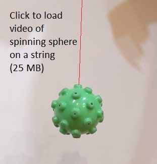
An image link to the video of spinning a sphere on a string to simulate the rotation and precession of a sphere on frictionless bearings. In the image, the string is highlighted in red for clarity.