A mathematical equation is defined by the presence of the equal sign, yet this sign breaks the symmetry of the underlying structure. More problematic, the equal sign is almost always used in practice as an assignment operator, that is, a more rigorous syntax would replace "=" with "↤" or "↦" as appropriate. But then the written equation defines not only a mathematical relation but also an informational relation of what is known and unknown, conflating the two in a manner that requires a complete re-write of the equation to solve for a different unknown. For instance, in all the major programming languages, a value is assigned to a variable by an expression like A=B+C, but what this really means is A↤B+C, where the arrow makes explicit the fact that B+C is a known (or calculable) value while A will be overwritten by this value. This syntax is carried over from mathematical instruction, where an equation like 5*x-3=2 is re-arranged into a form like x=(2+3)/5, which is really to say x↤(2+3)/5, because once having written the equation in this format there is no ambiguity about the right side so it defines the left and not vice versa. The shorthand of just using the same "=" symbol throughout all these cases covers up an important fact: algebraic manipulations to "solve an equation" are actually syntactic rather than mathematical operations. In other words, if we used a better syntax for mathematical expressions, we would not need to keep re-writing these expressions to "solve" for different vertices (and operations could be defined rigorously in terms of graph theory, as modifications of a network representing the structure of the equation system). This is the goal of Structural Expressions.
Readers interested in equation solving for engineering calculations should be aware of the software Engineering Equation Solver and MathCAD.
Consider again A=B+C. This is "solved" for A, such that A↤B+C, when B and C are known. If instead we have A and B known but C unknown, we have to re-write the equation into the form A-B↦C or C↤A-B. The mathematical purpose of the equation has not changed but now it looks completely different because the assumption on what is known or unknown has changed. I would like to specify the mathematical structure in such a way that it is independent of what is known or unknown and can be solved in an identical process for any configuration. This necessitates a manner of combining the vertices A,B,C in a way that preserves the symmetry of the structure. The equation actually has a hidden ambiguity: we can combine these as 1=(B+C)/A or as 0=B+C-A; we are taught to ignore the ambiguity by following standard algebraic (syntax) manipulations to "solve" for a single unknown to assign to. The linear combination has a higher symmetry here, so the structure of the equation A=B+C is sum0(-A,B,C), where the sum0() node imposes a requirement that all the vertices within its parentheses must sum to zero. This syntax is what I call a Structural Expression. Given sum0(-A,B,C), if we define A and B the node will solve for C, while if we define B and C the node will solve for A and so on. One might say "this is just a glorified calculator", but such a statement overlooks the power of the structural expression: in changing what vertices are known and unknown, there is no need to change the expression itself! So this is not just a calculator, but rather a calculator that intrinsically handles all the syntactic re-arrangements of algebra. In a fixed-assignment programming language (where one must write something like A=B+C to assign to A), making a change in what is to be calculated requires a complete re-write of the equation(s) (to be done by the programmer following algebraic rules). In a structural expression, this same change is very simple - just define the unknown vertex as unknown. The expression, representing the mathematical structure of the problem, remains unchanged.
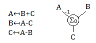
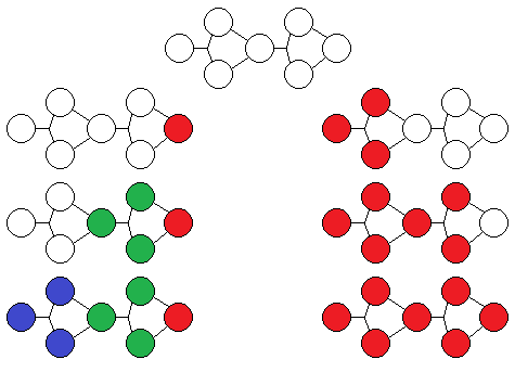
A comparison of the traditional equation and structural expression syntax. On left, there are three ways to write the equation A=B+C, solved for each vertex, and none of these equations make explicit the underlying symmetry. On right, the structural expression signifying a Σ0 node where all the attached vertices sum to zero; this expression remains the same regardless of what to solve for. Note the -1 on the connection to A, signifying this value is multiplied by -1 when evaluating the sum.
In a general manner, we may describe a system of equations using nodes and vertices, where nodes connect to vertices. A node of the same kind will perform the same operation on its attached vertices, and a vertex of the same kind will set all its attached nodes to an identical value. sum0() above is a node. In a sense, a vertex is an "equality node", in that its operation may be seen as an extension of the equal sign beyond two sides, from A=B to A=B=C=D if it were written with one equal symbol, or equal(A,B,C,D). However, because it is convenient to distinguish between numerical values of quantities (rather than between combinations of quantities), the typical approach is to use the name of a vertex as the equality relation. Even above this was implicit: A really means equal(A1,A2,A3) where A# represents unique appearances of A in different places in the system of equations. That is, instead of specifying a functional name like equal as in the case of nodes, we specify a unique identifier name like A for a vertex, knowing that its function is that of setting equality between all appearances of the unique identifier. If we use lines to represent vertices in a diagram, and allow lines to connect to each other to have an "extended vertex", then it is possible to draw a system diagram where a variable name appears only once. This makes the connectivity of nodes in a system easier to visualize. It should not be overlooked that such a node-vertex representation has wide applicability: electrical circuits, piping diagrams, processes and flows, node graph programming. Perhaps there is a statement here about the physical significance of such a representation.
Within the standard mathematical curriculum, I can think of two types of nodes where an arbitrary number of vertices may be combined: addition and multiplication. (There are also inverse-inverse / parallel addition and multiplication combinations, as well as other order analogues such as root of summed squares, and probably others I am not aware of.) Above I already introduced the Σ0 node where all attached vertices must sum to zero. Solving the node is simple: if there is exactly one unknown vertex, its value is such that when added to the rest of the known vertices the total sum is zero. If there are two or more unknowns, a solution cannot be found directly; because some of these unknowns may come to be defined by other nodes we may attempt solving this node again later. If there are no unknowns, then we may verify that all the known vertices actually sum to zero (or the node is over-constrained). For the multiplication node, which we may call Π1, all the attached vertices will need to multiply to 1, and the solution logic is analogous to the above. By attempting to solve each node in turn, assuming an algebraic solution exists, we will eventually reach the solution without having to rewrite the structural expression.
In engineering calculations, it is often useful to see the impact of some variable on the result of the calculation. This helps with both optimization and error propagation. For instance, when designing a beam of certain width, length, and height, which one of these has the most impact on strength and weight? If one of these is slightly off tolerance, how much will the quantity of interest deviate from expectations? To aid with this, each node is defined to solve not only for a numeric quantity, but also for the derivative of that quantity with respect to the known inputs of the node. To avoid double-counting, each known vertex is labeled as a "slope source", and then each node calculates the derivative in terms of any slope sources connected to it. Second and higher derivatives are not used because then combining multiple sources is no longer so simple. To put in mathematical terms, say a numeric node solves for x=f(y,z). We extend this to x+sy*dy+sz*dz=f(y+dy,z+dz), where sy,sz are slopes of the solution plane relative to the sources y,z.
This provides a robust technique that enables tracing the influence of calculation inputs on outputs while maintaining the straightforward nature of numerical solutions over symbolic solutions. It is not just taking a derivative, but rather referencing the result of a computation to an underlying source variable and combining such references. Some example relations are shown below; the uppercase letters represent numerically defined values while the lowercase letters represent small perturbations, the contents inside {} parentheses represent a single vertex value and the contents inside [] parentheses represent a slope. Note that all computations involving slopes may be categorized either as multiplying the slope by a constant or as adding multiple slopes together, thus they may be stored in computer memory as a number and a pointer to the source vertex. Applying an operation and its inverse will return the original slope to within numerical accuracy, without requiring the computer to keep track of operation history.
{A+[B*a]} + {C+[D*c]} = {A+C + [B*a + D*c]}
{A+[B*a]} - {C+[D*c]} = {A-C + [B*a - D*c]}
{A+[B*a]} * {C+[D*c]} = {A*C + [C*B*a + A*D*c]}
{A+[B*a]} / {C+[D*c]} = {A/C + [B/C*a - (A*D/C^2)*c]}
{A+[B*a]} ^ n = {A^n + [n*A^(n-1)*B*a]}
ln({A+[B*a]}) = {ln(A) + [B/A*a]}
exp({A+[B*a]}) = {exp(A) + [exp(A)*B*a]}
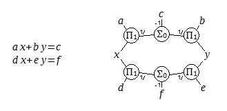
A structural expression for a linear system in two variables (x,y) and six coefficients, with equations typed on the left. Interestingly, when drawn this way, two equations turn into a single loop.
We soon run into a challenge - it may be the case that multiple nodes will have two or more unknowns, and yet a solution exists and should be found. This can happen even with quite simple equations, such as a two-variable linear system illustrated above: a*x+b*y=c, d*x+e*y=f. This may be solved directly (that is, each node will eventually have just one unknown to solve for) when we know (a,b,c,d,e,f) and either x or y. However if (x,y) are both unknown, there is not a node that can uniquely solve for them without knowing about the rest of the system beyond its immediate boundaries. The missing link is in combining the equations across one of the nodes such as a*((f-e*y)/d)+b*y=c or a*x+b*((f-d*x)/e)=c, which may be found by algebraic manipulation. Rules may be formulated that would allow determining such expressions from the structural diagram, but I couldn't readily find such rules. It may also be expected that in the general case the situation will not be so simple, and I am seeking a generally applicable algorithm that does not depend on a particular structure. For instance, a 3 variable system is illustrated below.
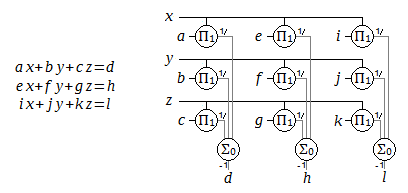
Equations and structural expression for a linear system in three variables (x,y,z) and twelve coefficients. The diagram has been drawn in a matrix form, but may also be visualized in 3D space with the sum nodes extending out of the page.
Thus we may end up with equation systems or (square) matrix equations: no single equation provides a solution for one unknown, but all the equations taken together define a solution for all the unknowns. It should be possible for the node approach to also find this solution. To avoid the need for complicated graph-reducing algorithms which could rearrange the nodes to isolate individual unknowns (which is how these systems are solved by hand, when they can be solved by hand), I instead take an approximation-improving iteration approach. This has the benefit of not constraining the structural expression to any particular form, including the ability to combine addition, multiplication, and non-linear nodes. An input system is processed into direct solution paths, solution regions, and unknown regions.
Originally, I hoped that it would be possible to solve the multiple-unknowns problem without looking at the entire system, that is, each node would only deal with its neighbors and improve the solution locally, and after enough time the global solution would be reached. The way this works is: given initial guess values for all unknowns, each node updates these values such that the node is satisfied and that there is minimal change in the values as measured by a Euclidean distance. The second condition is critical because it gives the node a history dependence and ensures that the steps towards a solution (if one exists) will become increasingly small over time. The justification behind the convergence of this implementation is given in the article Iterative Method for Solving a System of Linear Equations, Proc. Comp. Sci. 104 (2017).
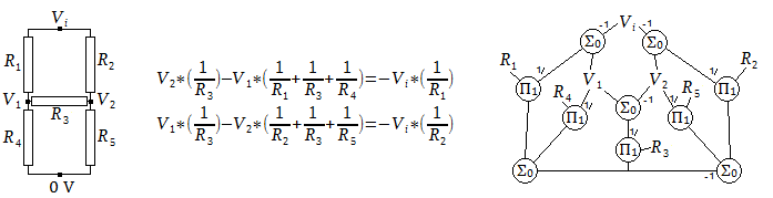
The voltage in a 5-resistor network, electrical schematic on the left, is solved by a system of two linear equations. These equations are indicated in the center (determined by applying charge conservation at V1,V2), along with the structural expression on the right. The structural expression clarifies the integrated nature of the two equations because the entire structure is connected, and also presents a solution path for any of the resistance values.
Such an implementation worked decently, but it would be easy to define a problem where the algorithm could get bogged down and take many thousands of iterations to reach a nearby solution. This was because the separation of equations into nodes, while making nice symmetric diagrams, separated the (nominally unified) informational content of an equation into disconnected entities. For instance in the 5-resistor network example above, if V1,V2 are unknown, then all 10 of the nodes would have two or more unknowns and would have to be iterated (with 10 total unknowns). On a surface level, a 2-variable system of linear equations has been changed into a 10-variable system, and the iterative approach is sensitive to such a change in dimensionality. For a change in a guess value to propagate, it would have to pass through multiple nodes, and without knowledge about the direction of information propagation, this effect becomes diffusion-like. If the iteration is accelerated, by having each node take multiples above 1 of its calculated step, the solution is reached slightly faster (hundreds of iterations instead of thousands), but then on other problems the accelerated algorithm becomes unstable. Maybe there is some clever way to solve systems locally, but I could not come up with one. Instead, I implemented an approach that would determine and enforce a particular direction of information flow when such a direction is available. This would further reduce a system to the smallest number of unknowns. For the 5-resistor network above, with V1,V2 unknown, this approach reduces the system to one unknown region which is solved in one iteration.
I also attempted to find a solution in terms of loops. The idea would be to define a set of loops through the unknown vertices and nodes, and update guess values by traversing around the loops. An important feature is that a loop may be traversed forward and backward, and the lesser change kept - then the individual loop may be guaranteed to be stable. This would be a step on the way to proving a solution algorithm to be generally stable, and maybe someone more mathematically inclined could make ground with this approach. I was not able to figure out how to extend the loop stability to an entire system. The number of loops that may be defined in a system grows rapidly with new nodes added, and it becomes difficult to mathematically justify which loops are the most important. I can say that picking loops at random, or using all of the loops, does not work: even picking the smaller change on each individual loop, the system diverges more often than not.
First, a direct solution is attempted. All nodes which have exactly one unknown (or a multiply-connected vertex which may be solved), are solved. In addition to the solved value, a derivative is stored referenced to a defining variable for sensitivity analysis. The solved vertex is then used to find new nodes (its attached nodes) to check for whether they can be solved. Eventually, either the entire system is solved, or everything except some unknown regions is solved. The unknown regions have two or more unknowns at each node. Fully disconnected unknown regions may be split into solution regions, and each solution region solved independently of others. From here, I will focus on a single solution region, which may contain multiple unknown regions.
Second, the unknown regions are to be represented in terms of one defining vertex per unknown region. In a system of equations, these are the (say) x,y,z variables that appear in each equation, however in the structural expression we do not know ahead of time which vertices should be considered as defining vertices (since their values may be either known or unknown). We pick an unknown vertex at random, and then check which nodes may be solved assuming this vertex is known. The resulting solved vertices have a value directly derived from the first unknown vertex, and are thus part of the unknown region defined by that vertex. We continue this process, adding vertices to the unknown region, until reaching nodes that cannot be solved: these nodes will either have multiple unknown regions incident, or will have one unknown region multiply incident. Therefore these nodes are added to a list of boundary nodes in the solution region. Next we pick another unknown vertex, and nucleate another unknown region defined by it. This is continued until all unknown vertices are in an unknown region.
One-way solutions make a difference in how an unknown region is defined. In the illustrated system (schematic only, external vertices are not drawn) as snapshots from top to bottom, if we start an unknown region from right to left, we end up with three unknown regions; if we start from left to right, we end up with one.
There is another challenge with generating unknown regions: one-way solutions. This may occur even when all nodes are invertible, because a vertex once solved may affect multiple nodes. For instance, if B=e(A), C=f(A,B), D=g(A,B,C) then an unknown region defined by A may be directly solved to find B,C,D. However an unknown region defined by C will not be directly solved in this manner because C=f(A,B) is not invertible with A,B unknown. Since above we have chosen vertices at random to define an unknown region, we may expect that some regions of the form {C} will be found. To resolve this, there is a need to join unknown regions when one may be defined by another. This ensures that the "most influential" vertex will be used to define an unknown region. When doing this, it becomes necessary to keep track of the reversibility of a solution path, such that a region may be joined from its defining side but not from a side which has passed through a non-invertible structure.
Third, we can now operate on unknown regions and boundary nodes. When every node can (in principle) define exactly one vertex, it can probably be shown that the solution region may be solved when the number of unknown regions equals the number of boundary nodes. Since we keep track of derivatives in node solutions, we can make a guess for each defining vertex set as a slope source, then solve each unknown region based on its guess value, and evaluate the boundary nodes in terms of values and derivatives referenced to the defining vertices. Then using the derivatives at the boundary nodes, it is possible to form a system of linear equations in terms of defining vertices, with one equation per boundary node. Because the derivatives are solved in each iteration, this linearizes an arbitrary system near the existing guess values.
Fourth, the linear equation matrix is solved (reduced row echelon form) to find the desired change in guess values. This change is added to the guess values defining each unknown region, and the unknown regions are solved again. This process is repeated until some convergence metric is satisfied. In this implementation, the metric is that in each node the difference from a desired solution is less than 1/100000 of the largest value of the connected vertices, and that after solving the matrix, each vertex value changes by no more than 1/100000 of its previous value in the final step.
Fifth, we complete the sensitivity analysis for solution regions by applying slopes from their influencing vertices. The influencing vertices are ones which give a direct solution that changes the boundary conditions for a solution region. In the 2-variable linear system shown earlier, the coefficients (a,b,c,d,e,f) are influencing vertices. What is the change in (x,y) when one of these is changed? The use of slopes enables this to be determined, since the linearized equation matrix is already in terms of the changes (dx,dy) (for instance) and the constants for the linear system solution will be in terms of (da,db,dc,dd,de,df). By rearranging the numeric values in the RREF operation and keeping track of which slopes come from which vertex, we obtain linear equations for dx=f(da,db,dc,dd,de,df) and dy=g(da,db,dc,dd,de,df).
It is often useful in engineering studies to run the same calculation with a few different values, for instance a range of beam widths or a set of material properties. Then, a known vertex may be specified with a list of values. A solution will be found for each entry in the list. Multiple vertices specified with lists will result in a solution for each unique combination of values. Multiple vertices specified with a table will result in a solution for each entry in the table. Units are also tracked and solved by nodes when possible.
In this paradigm, a system is defined in text format by having each line represent either a node or a vertex. A vertex is defined by its name, "=", value and units. A node is defined by its name, ":", vertices and constants. There is no requirement on line order - a vertex may be used in a node preceding its line definition. A vertex that only appears in node lines and does not have its own line definition is considered internal, so it is not included in sensitivity analysis or results printout.
// vertices: defined with a unique name, an equal sign, value, and units in [] brackets
// Name must start with an english letter, must not contain punctuation used for control sequences described below, may contain spaces and underscores
U = 5 [m] //a known value with units
V = [m^2] //an unknown value with known units
Z = // unknown value and units
// vertices with unknown value and units are defined implicitly in node statements
W = {1, 2, 3, 4, 5} [Kg] //a list of known values and units, result will include all combinations of list values
T = {1;1;5} [Kg] // a list of known values defined by endpoints and spacing, expands to the same list as above
S = {10, 11, 12} [m] @ Table1 // a row in a named table is specified using "@" and the table name
R = {20, 21, 22} [m] @ Table1 // result will include a solution for each column in the table
X = <1;0.1;10> [s] //a guess value with min and max bounds to solve by iteration method, units required
// Nodes: defined with a node name, a colon, and vertices or values separated by ',' and ';' characters, as required by particular node
// constant numeric values may be used which must start with a decimal digit, possibly including an 'e' for scientific notation, and required units in []
// vertex names which have not been declared before will cause an implicit initialization to unknown value and units
sum:U,V;W // U+V=W
product:X,Y;Z,V // X*Y=Z*V
power:A;2[];B // A^2=B
tangent:D;E;F // tan(D)=E/F
exp:G;H // exp(G)=H
distance:Q,R,S,T;U //Q^2+R^2+S^2+T^2=U^2
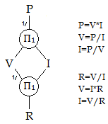
A structural expression for electrical voltage, current, power, and resistance, with six assignment-form equations that it encompasses directly. There are two Π1 nodes where all the attached vertices multiply to one; this expression remains the same regardless of what to solve for. Note the 1/ on the connections, signifying this value is inverted when evaluating the product.
The power dissipated by an electrical resistor, along with voltage, current, and resistance, are calculated: P=V*I, V=I*R. Any two quantities may be used to solve for the other two. This may be solved directly (that is, each node will eventually have just one unknown to solve for) when we know (V,I), (V,P), (I,P), (V,R), (I,R). However if we know (R,P) then (V,I) are both unknown, and an iterative solution is used (a guess must be provided). Unit conversion is not automatic, so [ohm] and [W] are defined with inline constants.
// vertices:
V=120 [V]
I=2 [A]
P=
R=
// Nodes:
product:V,1[ohm*A*V^-1];I,R
product:P,1[W^-1*V*A];I,V
The above system is solved directly with the results shown below. In addition to the computed values for power and resistance, their linear dependence on current and voltage near the solution point (slope) is found.
V = 120 [V]
I = 2 [A]
P = 240 [W]
	I : 1.2E+02 [W]/[A]
	V : 2 [W]/[V]
R = 60 [ohm]
	I : -30 [ohm]/[A]
	V : 0.5 [ohm]/[V]
For an end-loaded cantilevered beam, the deflection δ at the end is proportional to the load W and to the length cubed L^3, inversely proportional to the material's modulus E. It is also inversely proportional to the cross-section moment of inertia I, which for a rectangular beam of width w and height h is given by w*h^3/12. We may represent the two equations as two Π1 nodes with weighted connections. This is illustrated below.
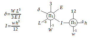
On left the equations for end-loaded cantilevered rectangular beam deflection, and on right the structural expression for these equations. Note the -1 and -3 on various connections signifying an exponentiation when calculating the product. As before, the structural expression does not emphasize a single vertex to solve for and highlights the underlying symmetry.
The system may be solved conventionally, in which case the two nodes allow for two unknowns distributed between them. The equations are written to find I from w,h, and then to find δ from the rest of the vertices. The structural expression makes no such preference. The code below shows how this system may be set up:
// vertices:
W=500 [N]
L=1 [m]
E=2e6 [N*m^-2]
I=
d=
h=0.5 [m]
w=0.25 [m]
// Nodes:
product:d,E,I,3[];W,L,L,L
product:I,12[];w,h,h,h
Evaluating the above, the second product node can solve for I, and then the first product node can solve for d. Note that units are also solved by the nodes in a similar manner: they must be identical in a sum node and they must multiply to unity [] in a product node. We receive the following output, noting from the slope values that deflection strongly depends on beam height, in agreement with engineering intuition.
W = 500 [N]
L = 1 [m]
E = 2E+06 [m^-2*N]
I = 0.002604 [m^4]
	h : 0.016 [m^4]/[m]
	w : 0.01 [m^4]/[m]
d = 0.032 [m]
	h : -0.19 [m]/[m]
	w : -0.13 [m]/[m]
	L : 0.096 [m]/[m]
	W : 6.4E-05 [m]/[N]
	E : -1.6E-08 [m]/[m^-2*N]
h = 0.5 [m]
w = 0.25 [m]
Let's say instead of solving for I,d we now want to solve for w with a known d. If we had done the above with assignment-form equations, we would be rewriting both of them. But with the structural expression we just change the unknown vertices to a blank and the known ones to a value:
// vertices:
W=500 [N]
L=1 [m]
E=2e6 [N*m^-2]
I=
d=0.01 [m] // this is now known
h=0.5 [m]
w= [m] // this is now unknown
This gives the result:
W = 500 [N]
L = 1 [m]
E = 2E+06 [m^-2*N]
I = 0.008333 [m^4]
	d : -0.83 [m^4]/[m]
	L : 0.025 [m^4]/[m]
	W : 1.7E-05 [m^4]/[N]
	E : -4.2E-09 [m^4]/[m^-2*N]
d = 0.01 [m]
h = 0.5 [m]
w = 0.8 [m]
	d : -80 [m]/[m]
	h : -4.8 [m]/[m]
	L : 2.4 [m]/[m]
	W : 0.0016 [m]/[N]
	E : -4E-07 [m]/[m^-2*N]
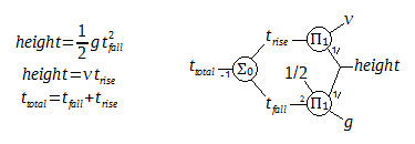
The equations and structural expression for the time of sound after a fall, with gravitational acceleration g and speed of sound v. Note the small numbers on various connections signifying an exponentiation on the product or negation on the sum nodes. Compare the loop shape of the quadratic equation to the loop seen earlier with the 2-variable linear system - the diagram makes it clear that the quadratic equation, although written as one equation, cannot be solved directly.
When an object is dropped from a high point and hits the ground, an observer at the drop point will hear this sound after a time defined by the duration of the fall and the speed of sound over the distance of the fall. Setting the expected drop height as unknown and the time of sound as known makes a quadratic equation which is linearized and solved iteratively, reaching a solution in 3 to 4 iterations for each time value. To find the drop height at multiple values of time, the list syntax is used. An approximation (the height ignoring the speed of sound) is used as the initial guess value for height to speed up the convergence. The underscore assignment =_ is used to define a constant value which will not be included in sensitivity analysis, and t_rise,t_fall,height_guess are internal vertices.
g=_9.8 [m*s^-2]
v=343 [m*s^-1]
t_total={0.5;0.5;10} [s]
height= <height_guess;0.1;1000> [m]
product:0.5[],g,t_total,t_total;height_guess
sum:t_rise,t_fall;t_total
product:0.5[],g,t_fall,t_fall;height
product:t_rise,v;height
The result for t_total = 1 [s] is shown below. The full results table is presented at the end of the Minimum Rope Tension article.
v = 343 [m*s^-1]
t_total = 1 [s]
height = 4.765 [m]
	t_total : 9.4 [m]/[s]
	v : 0.00038 [m]/[m*s^-1]