This project came from a need to import real photos of components as texture files into a CAD program, but the finished program obviously has the potential for much wider applicability. When taking a photo of an object, it is difficult to get a perfectly aligned shot where the object surface is parallel to the camera. Also, if online or manufacturer-provided photos are used, they are generally taken at an angle to show more faces of the object. The idea of this program is to take these off-angle photos and transform them such that a particular surface in the photo appears to be parallel to the camera. Then, this parallel surface can be used as a texture file, for pixel distance and angle measurement on the surface, or as a starting point for further analysis. The program is written in C# and is based on the .NET framework.

An example of the image straightener in action. Left side is the original photograph of a poster, and right side is the transformed photograph to make the poster appear as though it was photographed squarely.
The program operates largely through a click-and-drag interface. We note a few limitations before starting:
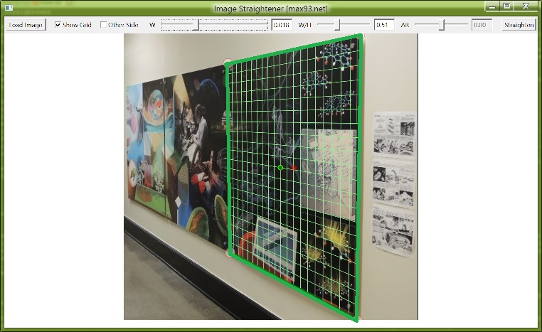
As an example, we will straighten the following photograph of three posters. The posters are square, which will help determining the aspect ratio:
The original photo of posters. It is desired to see the posters from the perspective of standing directly in front of them.
Press the Load Image button and select the original image. It will show up in the window along with a red selection rectangle.
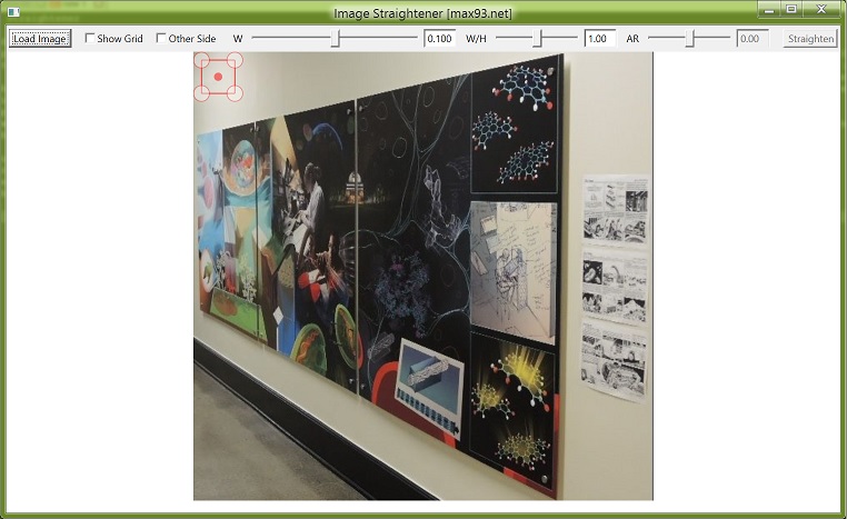
An original image is loaded in the program.
Drag each of the red rectangle corners to outline a rectangle in the image. Also, you can drag the central red dot to move the entire rectangle outline. The program is not guaranteed to work if you switch the order or orientation of corner points while dragging (that is, top left->top left, etc). It is not guaranteed to work otherwise either, but there is probably a higher chance of it working. If you drag the corners outside the image area or want to start over with the selection at any point, click Load Image and then Cancel out of the dialog. That will reset all UI elements to their original settings.
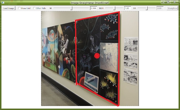
The red rectangle outline is dragged to outline a rectangle in the image. The red lines were drawn thicker in this photo for clarity.
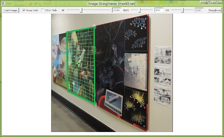
Click the Show Grid checkbox, which will draw a green grid showing the plane containing the red rectangle. Sometimes the grid will not be visible or will appear 'broken', in which case adjust the W slider so that the grid fits within the window. The edges of the grid have a dark green outline.
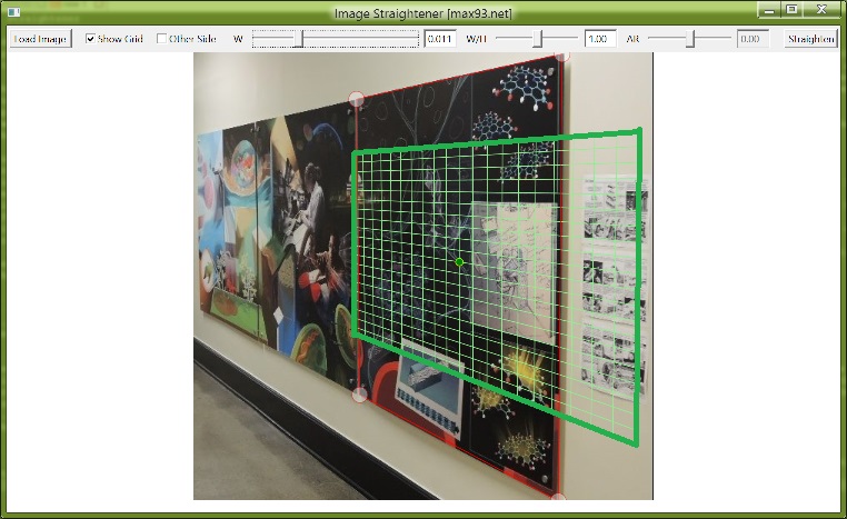
The green grid shows the plane containing the outlined rectangle, once W has been adjusted. The outer edges were drawn thicker in this photo for clarity. The grid should outline squares in the image, if it outlines rectangles the output image will be stretched either horizontally or vertically.
If the grid looks like it outlines squares in the off-angle plane, then there is no need to adjust the W/H setting. It is computed internally and is generally accurate for images that are only slightly off angle. However sometimes the setting is incorrect, in which case the grid appears to be rectangular (as in this example). You might first try the Other Side checkbox, which will compute the grid in a different manner. If that is still not accurate, adjust the W/H slider to make the grid appear square. Since it is known that in this example the posters are square, I will try to match the grid outline to the poster outline.
To do this, it will not be sufficient to adjust W/H. By default the grid origin is at the red rectangle center-point, but it can be moved anywhere in the image by dragging the green grid origin point. This has been done below to match the grid to one of the posters. Note that when the settings are correct, the grid origin can be moved to any other similar rectangle in the image and the grid will match it automatically.
The W/H setting has been adjusted to match the grid to the square poster. The grid origin was moved to the poster center. If there is not a square in the image, an adjustment can be made by eye, or the automatically calculated setting W/H=1 can be used.
With the correct W and W/H settings, the grid will automatically adjust to all similar sized objects when the grid center is moved.
The dark green grid outline shows the part of the image that will be transformed to the output image. It can be moved within the light green grid by the AR slider, and along with the W slider and grid origin a selection can be made of the desired transformation area.
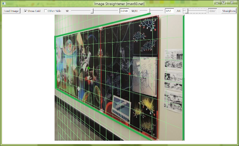
The grid covers the desired image area to be straightened, and the dark green outline determines a rectangular transformation area within the square grid.
Click the Straighten button to transform the image. Note that the Straighten button is only available if the Draw Grid checkbox is checked, and the grid was drawn without errors (indicating properly chosen constants).
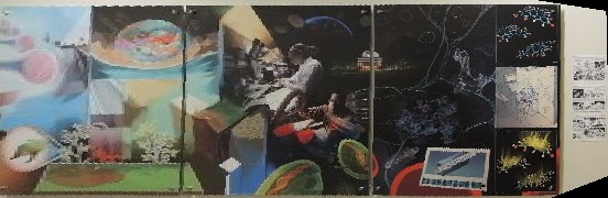
The output image shows square posters as desired.
Here are some other comparisons of the before/after poster images, showing the effectiveness of the algorithm:
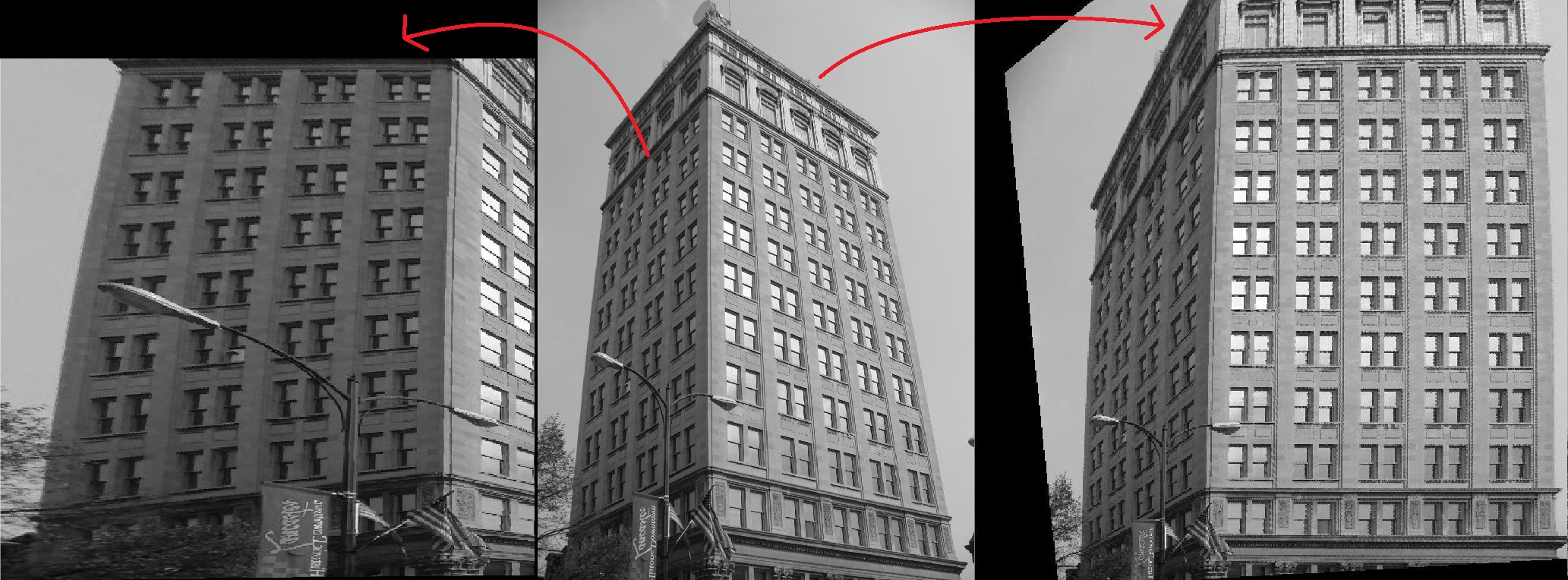
This photo of a building has been straightened in two ways, on both of the walls making up the corner that was photographed. The left side shows some effects of lens distortion since the straightened image has a bit of curvature.
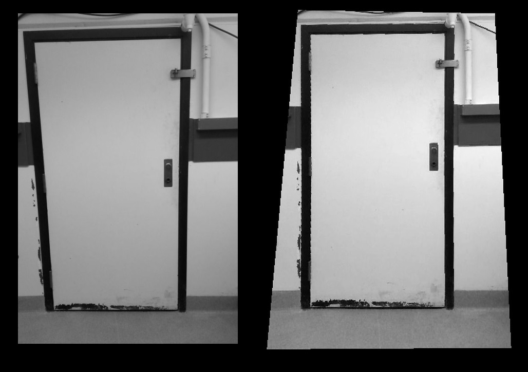
The left photo of a door has been straightened on the right so the door is nearly rectangular. Note the effect on the border of the original photo, it is as if one held the photo at an angle.
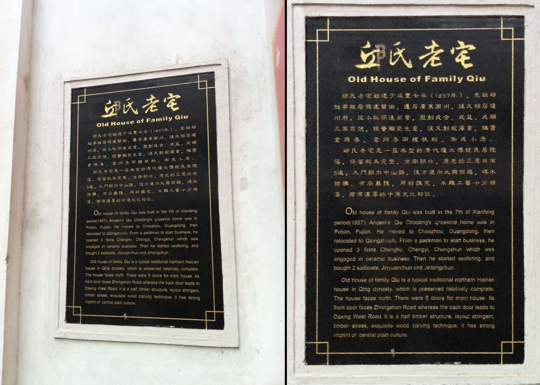
A practical example shows how a photograph of a sign may be straightened to be more readable.
We start with the concept of a projection, or the way a real physical object can be represented as a 2D array of pixels which is the input photo. This understanding is necessary if we are to attempt to recreate the appearance of the real object at a different orientation. Since this program attempts to straighten photographs, let us first review the way a camera operates.
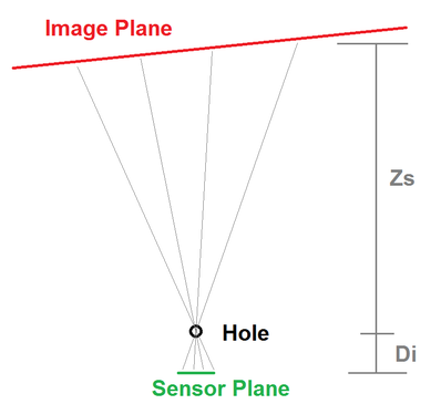
A schematic of camera operation viewed from above.
In the camera, what is imaged is a variation of photon angle. We take the classical optics view that photons travel in straight lines, and then place a pinhole in front of the rectangular pixel sensor containing square pixels (a lens is a fancier version of a pinhole that can collect a wider range of photon angles given a location of the imaged object, which brings the need for focusing when a lens is used). The apparent size of an object on the camera sensor is based not just on the size of the object, but also on the ratio of the distances between the pinhole and object, and pinhole and sensor plane. Thus we can see objects that are hundreds of meters in width even though the eyeball diameter is only a few cm.
Furthermore, the pixels are equally spaced in the horizontal and vertical directions on the camera sensor. This means that, given an imaging plane that is parallel to the camera sensor, a square at any location in the imaging plane will map to the same sized square in terms of pixels. This is not always true, for instance the 'pixels' in the retina are on a spherical surface, so squares farther away from the center will appear smaller and slightly warped compared to directly centered squares (as with the fisheye lens).
To put the problem in mathematical terms, we write the function that projects from the real 3D space (x, y, z) to the pixel space (px, py) with the pinhole at the origin (0, 0, 0) and the pixel plane parallel to the XY plane and passing through (0, 0, -Di), with the pixel (0, 0) also occurring at that point. Realistically, the image in pixel space will be flipped horizontally and vertically after passing through the pinhole, but here we use an imaginary 'reversed' pixel plane where this flipping does not occur. This corresponds to an absence of a multiplicative factor of -1 in the formulas for px and py:
px=x/z*Di
py=y/z*Di
This is a nonlinear transformation, meaning that it cannot be reversed. This makes sense since the transformation condenses three variables into two. This forms the basis for many photo tricks and illusions, which if done skilfully cannot be distinguished from a 'real' image, but are only effective with a particular orientation of the camera pinhole and sensor with respect to the rest of the scene.
Next, we need to consider what a general rectangle will look like in 3D space. The rectangle will be in a particular 2D plane within the 3D space, and we let the origin of this plane be at its intersection with the z-axis at the point (0, 0, Zs). Such a definition favors low angle offsets from parallel, which is also the best case in terms of pixel resolution (otherwise near the horizon/vanishing point a few pixels become mapped to arbitrarily large areas, leading to very blurry images).
First, the rectangle is defined with its bottom left corner at (Px, Py) in the 2D plane described above, and its top right corner at (Px+w, Py+h). This implicitly sets dPx=0 and dPy=0 along the lines of the rectangle. These coordinates will be termed as 'system 1'. The mapping from system 1 to the 3D system is simply (Px, Py, Zs).
Second, the general rectangle can be rotated within this plane by angle theta_r. A unique rotation, given variable w and h, will be in the range of 0 to 90 degrees, or -45 to 45 degrees. This will be considered system 2. From system 1 to system 2 is a regular 2D rotation matrix:
x2=cos(theta_r)*x1-sin(theta_r)*y1
y2=sin(theta_r)*x1+cos(theta_r)*y1
z2=z1
Third, the entire plane is rotated about a particular axis so that it is tilted towards or away from the camera. This is the penultimate representation, system 3. One angle, theta_a, specifies the direction of the axis about which the plane is tilted (alternately, the axis which remains in-plane after rotation). A second angle, theta_o, is the out-of-plane rotation about the earlier defined axis. Combining some 3D rotation matrices we find the following relation between system 3 and system 2 coordinates:
(math)Fourth, the rectangle coordinates of system 3 are projected onto the camera sensor, the pixel plane, which is system 4. The transformation was already described above:
x4=x3/z3*Di
y4=y3/z3*Di
The first two transformations are linear, and therefore can be written as matrices and multiplied together to get a combined transformation. Performing the lengthy calculation results in the following matrix:
[matrix]To make the problem easier to read, we define variables to represent the quantities in the above matrix:
a=..
b=...
Then we have
x3=a*x1+b*y1
y3=c*x1+d*y1
z3=e*x1+f*y1+Zs
And applying the final nonlinear transfomation to these expressions, we obtain a Mobius transformation:
x4=(a*x1+b*y1)/(e*x1+f*y1+Zs)*Di
y4=(c*x1+d*y1)/(e*x1+f*y1+Zs)*Di
We can see that whereas in the first system the rectangle lines are parallel to the x and y axes, in the pixel plane the lines can be at any angle as determined by the six constants a-f, which are in turn based on the three rotation angles theta_r, theta_a, theta_o as well as Zs and Di. We assume Zs=Di=1, since there are still free variables in the rectangle width and height that can set the proper scaling, so seven variables remain (3 angles and 4 rectangle coordinates). The original hope for this program was to determine the parameters describing the plane in 3D space based just on the outline of a rectangle within the pixel plane. However, the prospects for such a solution do not look good, partially because of the inability to invert the last nonlinear transformation, and partially because of the difficulty in finding appropriate sine and cosine terms for the rotations. I attempted a brute force solution where a number of rotation angles are tried to see if an appropriate set of constants is matched, but the results were not satisfactory - the problem does not seem to be solved by something like Newton's method because the space is not really Euclidean.
The other alternative is to solve for the six variables a-f. However, there is no straightforward solution since the six variables are related by their trigonometric definitions above. Instead we will need to try another approach that extends beyond the scope of transformations.
For instance, we can take the limit of x1 to infinity and y1 to infinity. We see that this yields values for two points in system 4:
x1->inf: (x4, y4)=(a/e*Di, c/e*Di)
y1->inf: (x4, y4)=(b/f*Di, d/f*Di)
From here, adding a few postulates about mapping lines onto lines and so on, we can prove the validity of the idea of vanishing points as used in perspective drawings (at least in their similarity to photographs). Fortunately, we can make use of the above expressions directly since in the rectangle outline we will have two lines that change only in the x1 variable, and two lines that change only in the y1 variable. Therefore the intersections of the two pairs of opposite lines in the rectangle as it appears in system 4 coordinates directly give use the points a/e, c/e, b/f, d/f (with a known value for Di). All that remains is to find the values of e and f for a reverse projection to be possible. However once again this proves to be challenging or impossible within the given constructs. Trying to find either the slopes of lines in system 4, or their coordinate projections, or any other limits to infinity, all gives results in terms of the fraction e/f or e and f independently.
Trying out a few different values for e and f with a known set of the other 4 ratios, results in grids with variable spacing along the system 1 x- and y-axes (in other words, e and f set the extent of how stretched out a square appears to be along the horizontal and vertical directions). We can combine the e and f values to get (say) the ratio e/f and f, where the ratio determines the aspect ratio of squares in the grid, and the remaining variable determines an absolute magnification. We can generally get rid of the absolute magnification and set it based on the number of pixels in the image, but the e/f ratio remains elusive. In the program, the f value is set by the W slider, and the e/f value is set by an internal formula (see below) along with a multiplicative factor from the W/H slider, to allow correction of imprecise solutions. Finding the values of e and f requires recognition of the trigonometric relations between all the variables a-f. Instead of doing all that work, we assume knowledge of a point where both x and y go to infinity:
(x1, y1)->inf: (x4, y4)=((a+b)/(e+f), (c+d)/(e+f))Then the slope of the line from the origin to that point is dy/dx=(c+d)/(a+b). We can solve for e/f knowing this quantity, by using the known ratios a/e, c/e, b/f, d/f as follows:
s=dx/dy=(e*a/e+f*b/f)/(e*c/e+f*d/f)
e(c/e*s)+f(d/f*s)=e*a/e+f*b/f
e(c/e*s-a/e)=f(b/f-d/f*s)
e/f=(s*d/f-b/f)/(a/e-s*c/e)
Furthermore from some more approximations we find that s~=tan(pi/4-theta_r)~=tan(pi/4-theta_x), where theta_x=atan2(x_xinf, y_xinf) and (x_xinf, y_xinf) are the coordinates of the point where x1 goes to infinity. We can then solve for s and subsequently for e/f. The Other Side checkbox simply alternates between using (x_xinf, y_xinf) and (x_yinf, y_yinf) points in the atan2() function, since the underlying assumption is that rotation does not exceed 90 degrees.
This is the approach used in the program to set the default e/f ratio, and while numerically it works, its mathematical foundation is questionable which is the reason the W/H slider is necessary. This is a manifestation of the sensitivity of the mapping, where from the above brute force approach even a small rotation angle difference of 5 degrees leads to a factor of 2 difference in the W/H factor. Clearly as the infinity (vanishing) point gets closer to the image, the ratio becomes more sensitive to the way the rectangle is outlined.
Finally we define an inverse transformation to enable the solution of where the grid origin should be in system 1 coordinates based on where the grid origin is dragged in system 4 coordinates (knowing the 6 transformation variables). This is a straightforward solution of a 2x2 set of linear equations:
x1=(d*x4-b*y4)/((f*c-d*e)*x4+(b*e-a*f)*y4+d*a-b*c)
y1=(c*x4-a*y4)/((d*e-f*c)*x4+(a*f-b*e)*y4+b*c-d*a)The executable is available here. The installer file (which will also install .NET framework if it is missing) is available here. The source code is available here.