Sound is a large part of our everyday experience (music, communication, tracking), which made me curious to better understand how sound works - how sound waves propagate. This topic is usually covered in high school physics as an example of a 'simple wave' (along with water waves, neither of which are simple) but such introductory coverage has some shortcomings and leads to an inaccurate mental image. For instance, it is often claimed that long wavelength sound will diffract to a greater extent than short wavelength sound, in other words that short wavelengths are more directional. Why does this happen? Why are loudspeakers shaped in a specific way, and why do many wind instruments have an expanding horn at the end? How are sound waves reflected and diffracted in a room or around objects? Such questions may be answered with a numerical model of sound propagation, which here is loosely based on an elastically colliding gas model.
Since sound propagates in air, to better understand sound propagation it is necessary to model air in an accurate way. The ideal gas model describes air as molecules that collide elastically with the container walls but do not interact with each other. This can supply relations like PV=NRT but does not explain the Maxwell-Boltzmann distribution or sound wave propagation. In this model, sound waves would be individual molecules going faster than normal, so diffraction in the usual sense will not occur. The wave speed is also not constant, as pressure peaks are transmitted faster than pressure troughs. Finally, assuming no collisions seems to be in contrast with the real system - air is approximately 1000 times less dense than solid matter, meaning an imaginary cube surrounding a single molecule is only 10 times bigger on each side than the tight packing in solid matter. Even with the reduced density, there are perhaps 5e16 molecules in a cubic millimeter - there are plenty of opportunities for intermolecular collision! (Chemical reactions in gases is evidence that collisions actually occur, at least if gas is viewed as particles)
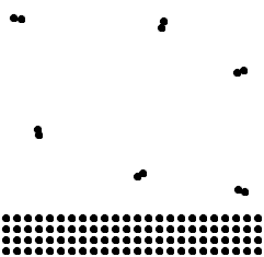
A mostly to-scale comparison between a solid (bottom) and a gas (top) assuming a 1000 decrease in density. A similar decrease will occur in the third dimension (out of the page). Elements that are not noble gases form molecules of 2 (sometimes more) atoms at standard condition.
Instead of the ideal gas model, I will use a more realistic 'elastic collision model' (kinetic theory of gases), in which molecules collide elastically not only with the walls but with each other. One question is, will this lead to a Maxwell-Boltzmann velocity distribution? In fact it does - it is possible to get the Maxwell-Boltzmann distribution with only Newton's laws and a large number of elastically colliding particles (which can start in any random distribution that leads to collisions between particles). Observing the behaviour of molecules in this model gives hints about the required characteristics for a sound wave propagation model - which unfortunately cannot be particle-based because of the huge number of molecules in macroscopic size boxes as mentioned above (there are particle-based models that represent many molecules with each virtual particle, such as smoothed particle hydrodynamics, but these are beyond the scope of the article).
Because of the many expected collisions, the model is implemented numerically rather than solving analytically. Molecules are represented as spheres, so there will be a discrepancy in heat capacity (molecules can rotate and store heat energy that way - molecules with high moment of inertia are used for quenching electric arcs) which should not affect the conclusions. Each particle has a 3-coordinate vector location and velocity, and a constant particle radius which defines when collisions with other particles occur. When two particles' locations are within two particle radii of each other, the particles are processed as an elastic collision. Only two-particle collisions are considered; when multiple particles collide at the same time the code will treat it as a sequence of two-particle collisions one after the other.
Particle motion is simulated explicitly as a function of time, so with the particle location vector x and velocity vector v the update is simply x = x + v*dt. The elastic collisions occur in 3D. All particles are assumed to have equal mass, so the result of a collision is the exchange of any velocity component that is along the collision line (the line passing through the colliding particles' center locations). The obvious approach is to determine the angular orientation of this line using trigonometry (sin/cos) but a faster approach is available from vector algebra: vector projection, in which the component of velocity along the collision line is calculated by projecting the velocity vector onto the collision line vector. The result of a projection is a scalar, which then needs to be multiplied by a unit vector to get the vector velocity that is exchanged between particles. Two remaining orthogonal velocity vectors are not exchanged by the collision.
collision_v=location1-location2 //collision vector is between the particle centers
collision_uv=collision_v/magnitude(collision_v) //change to a unit vector
v1_proj=dot(velocity1, collision_uv) //project particle 1 velocity onto collision vector
v2_proj=dot(velocity2, collision_uv) //project particle 2 velocity onto collision vector
A useful mental image is a pool table (this is not perfect, since balls have angular momentum and can be slowed by friction). If a ball strikes another ball 'head-on', all of its velocity is along the collision line and thus gets transferred to the other ball (also seen in Newton's cradle). If a ball strikes another ball with a 'glancing' hit, only some of its velocity will be transferred to the other ball, and the two will separate in a Y-shaped motion. The code for the particle simulation can be downloaded here.
2D systems can be simulated by setting the location and velocity in the Z direction to be zero for all particles. The boundaries are repeating, so a particle exiting the simulation area to the left will re-enter from the right, representing an 'infinite' plane. Here is what that looks like:
2D elastic collision system, with 100 particles starting as randomly distributed in position and velocity. The first 50 iterations are shown.
It is hard to tell what is going on when there are so many particles interacting, so to get clearer results from the model I keep track of the particles' parameters over time and plot histograms. Still the underlying mechanics are purely Newtonian. I track the particles' velocity magnitude as a function of time. Initially, the particles are placed at random locations and with randomly oriented velocity vectors all of magnitude 1. So at the start, the histogram of velocity magnitudes has all 100 particles shown as velocity 1. As the particles are allowed to collide with each other, a specific distribution develops, as shown below. This distribution is independent of starting velocity distribution (except for extreme cases like uniform velocity so no collisions occur). Even with initially ordered particles, one collision is enough to set off a 'chain reaction' of further collisions and increasing disorder approaching the shown distribution.
A 2D particle velocity magnitude distribution that is effectively independent of initial velocity distribution (here initial velocity is 1 for all particles). The image shows the result of 5000 iterations on an initial system where all velocities are 1.
In the resulting distribution, a fraction of the particles consistently has velocity between 0 and 1, while another fraction has velocity as high as 3. How could a particle go three times faster than its initial velocity, solely as a result of elastic (velocity-exchanging) collisions? This must be due to the dimensionality of the problem - repeated glancing collisions can slow down or speed up a particle beyond the speed of the particles with which it collides, since only some component of velocity is exchanged. Momentum and energy are still conserved when summed over all particles. If the problem were 1-dimensional, the particles could only keep their original velocities in elastic collisions, and not get faster or slower. Logically, then, the distribution should be different in 3 dimensions.
Changing the simulation to 3D only requires the initialization of a non-zero Z location and velocity since the vector algebra remains unchanged. Looking at the time evolution of the particles is interesting but again is hard to interpret for clues about overall behavior.

A 3D elastic collision system with 100 particles. From this explicit representation it is even harder to tell what's going on than with the 2D case. The first 50 iterations are shown.
The evolution of the histogram of velocity magnitudes in the 3D system is similar to the 2D case, approaching a specific distribution regardless of the initial distribution (in this case, all particles are initially set to velocity 1 uniformly distributed in 2-theta solid angle (all 3D directions), but many others were tested with the same result). The resulting distribution is noticeably different from the 2D case, in having a sharper dropoff toward lower velocities and a slight decrease in the high velocity 'tail' end, both of which contribute to a slight increase in the middle section of the distribution (surrounding the initial velocity 1).
A 3D particle velocity magnitude distribution in an elastic collision system approaches a specific distribution regardless of the starting point. The image shows the result of 5000 iterations on an initial system where all velocities are 1.
This is, indeed, the Maxwell-Boltzmann distribution that is often taken as a starting point in the ideal gas model. It is satisfying that this distribution has a mechanical explanation, which to me is more convincing than the more abstract energy equipartition argument. For the Maxwell-Boltzmann distribution it is known that the temperature relates to root-mean-square speed as RMS_speed = sqrt( 3*R*T/M ), so it is possible to adjust these parameters in the model to determine the equivalent temperature of the system, resulting in good agreement between the model and the analytical solution.

Three initial velocity magnitudes (0.5, 1, 2) were used in the simulation, which match up very well to the Maxwell-Boltzmann distribution given an equivalent temperature based on RMS speed.
The importance of a 3D simulation is shown by the mismatch between Maxwell-Boltzmann and a similar 2D simulation. 2D particles approach a different distribution, which ought to be physically testable in systems such as monolayer films.

Mismatch between Maxwell-Boltzmann distribution and a 2D particle model with initial velocity magnitudes of (0.5, 1, 2) similar to the 3D case above.
In this model, for information to travel from one spatial region to a neighboring one, particles have to physically move between regions. What happens when fast-moving particles enter an area filled by slow-moving particles? The ensuing collision eventually distribute the momentum among all particles. In the process, the energy of the incident particles becomes spread among all 3 dimensions, even though initially those particles were only traveling in one direction. This is how sound waves spread, and why Huygens' principle works for describing sound diffraction. In the next simulation, half of the randomly placed particles have velocity of 2 in the X direction only, while another half have 0 velocity. After a few thousand iterations, it is found that most particles have nonzero velocities in both Y and Z directions, although at the beginning none of the particles was traveling in either Y or Z!
The first 50 iterations with 50 moving particles and 50 stationary particles initially, showing eventual momentum and energy transfer from the moving to the stationary particles.
In other words, after about a thousand collisions per particle the initial direction of wave propagation (X in the above example) is effectively lost - the particle momentum is equally distributed in X, Y, and Z directions (except for a decreasing linear offset in X to maintain a constant sum of all particles' momenta). The histogram below illustrates the distribution of particle velocities in X, Y, and Z as iterations take place. In X, initially half of the particles have velocity 2 and the other half 0. In Y and Z, initially all the particles have velocity 0. As collisions take place, the Y and Z distributions spread out but remain centered at 0, while the X distribution takes on a similar appearance to Y and Z but is centered at 1 (average of 0 and 2) such that total X momentum is not changed. This can take place while conserving both total momentum and total energy since momentum is proportional to V while energy is proportional to V^2.
A histogram of the X, Y, and Z velocity components in the system with initially 50 moving and 50 stationary particles. The evolution takes place over 5000 iterations.
From the above, we can greatly simplify the model and instead of using individual particles, use properties of a certain spatial region (box) of particles to represent them. We saw that the velocity distributions in X, Y, and Z tend to become the same shape, with a linear offset to conserve momentum. So making the assumption that collisions between particles happen much faster than overall sound propagation (such that we can evaluate entire regions assuming they have already attained their 'steady state' momentum distributions), all we need to describe a region of particles is four variables: the magnitude of 'spread' in the velocity distribution, and the 3 linear offsets of the velocity distribution in each axis. For the individual velocity components (as opposed to magnitude, above) this spread is a normal distribution (proportional to exp(-x^2)) with standard deviation proportional to temperature.
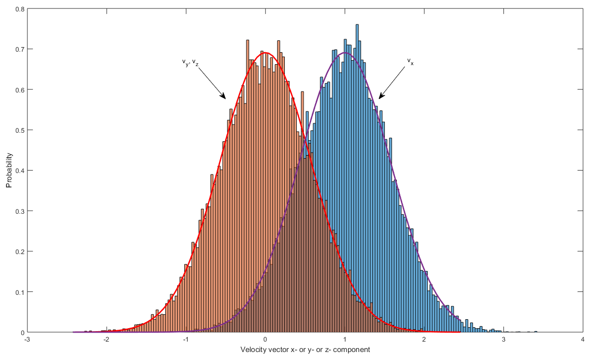
The limiting distribution for the X, Y, and Z velocity components in the system with initially 50 moving and 50 stationary particles. This is measured after 10000 iterations. Normal distributions with average of 0 and 1, and standard deviation of 0.577 (based on Maxwell-Boltzmann temperature definition) are overlaid to shown match of simulation and theory.
From the Maxwell-Boltzmann distribution we already know that the magnitude of spread of the velocity components is a direct indication of temperature - a wider spread, corresponding to larger achievable velocities, occurs at higher particle-averaged temperature. So all we need to describe a box of particles after many inter-particle collisions is a temperature scalar and a linear velocity vector. From PV=NRT, since the box volume is taken as constant, we can equate the qualitative function of pressure and temperature assuming the number of particles (density) is also constant. In this case V, N, and R are constants so P and T are proportional as P=T*(NR/V). This implies that pressure waves are also temperature waves, with the high pressure regions being at a slightly higher temperature than the low pressure regions. Indeed this is the principle used in thermoacoustic engines. It is a bit surprising at first sight that density should remain constant; for this we assume it is not molecules but the molecules' momentum which is transferred between adjacent 'boxes'. In order to use this assumption, we have to limit the study to 'small signals', that is typical listening-level sounds as opposed to (1) high amplitude low-frequency signals, (2) high-frequency signals, (3) shock waves. When the signals are not small, the molecules are transferred between 'boxes' along with their momenta, so parts of the wave travel at speeds other than the nominal speed of sound, introducing non-linearities such as wavefront pile-up and energy dissipation as heated air. These effects are used to advantage in ultrasonic directional speakers.
In conclusion, the elastic collision model along with the small-signal assumption leads to the possibility of representing sound as the transfer of pressure (or temperature) along with a velocity vector between adjacent 'boxes' filled with colliding particles. This greatly simplifies the computational effort required since only 4 variables represent a whole box of particles, so simulations of sound on practical scales can be carried out.
To simulate sound propagation in large spaces, we imagine many 'boxes' from above to be stacked adjacent to each other, covering the simulation space. At each box center we can define a local pressure, and at each box edge we can define a local velocity component. Since the above simulation shows that initially diverse particle distributions will tend to become the same shape, it is tempting to simply average neighboring pressures and velocities for the sound simulation. While this leads to a steady state pressure distribution it does not show observed sound propagation, since the sound wave in the averaging model quickly dies out as it travels farther from the source - even in 1D. This is because the earlier conclusion of reaching the same distribution describes the equilibrium state of the system rather than how that state is approached; we should not be too surprised that the resulting model does not accurately describe propagation.
Instead, we recognize that any transport of pressure or velocity between boxes takes place by individual molecule collisions. Specifically, a molecule must be traveling towards the box boundary in order to collide with a molecule from the adjacent box. If one box is at a higher pressure than the adjacent box, its molecules will be traveling faster in all directions - including towards the adjacent box - so from the adjacent box's point of view there is a velocity transfer from the high pressure (HP) box to the low pressure (LP) box. As collisions between these molecules in these boxes take place, only those of the HP box's fast molecules traveling towards the LP box will be slowed down, while the remainder retains their faster velocity. Thus, even if there is no net velocity of the air initially but only a pressure difference, a velocity component arises as the pressure equilibrates. Since pressure exerts a force, or equivalently an acceleration or dv/dt, we write this explicitly as:
dP/dx = -dv_x/dt
dP/dy = -dv_y/dt
dP/dz = -dv_z/dt
It seems that there should also be a contribution of the pre-existing (v_x, v_y, v_z) vectors in the above equation. However that would again jump ahead of the propagation and attain an equilibrium state too rapidly. Instead the role of the velocity vector is taken to impact the pressure. If there is a high velocity transfer from both the left and right sides of a box, the pressure will increase. But if there is a velocity transfer in from the left and out from the right, the pressure will stay the same. As before, the only velocity component that can be transferred on either the left or the right side is the component normal to that boundary plane. Thus we have spatial derivatives of the form dv_x/dx, dv_y/dy, dv_z/dz in accounting for the change in pressure.
dP/dt = -( dv_x/dx + dv_y/dy + dv_z/dz )
Taking V as the velocity vector, the first set of equations can be written as grad(P) = -dV/dt and the second one as dP/dt = -grad(V). These two can be combined (by integrating grad(V) to get V, substituting into dV/dt, then differentiating) to make the velocity implicit: grad2(P)=d2P/dt2. This is the acoustic wave equation, without the constants since this has been a rather unrigorous derivation. In any case this equation, with appropriate boundary conditions, is what needs to be solved to get a model of sound propagation. From this equation we might get a '1D acoustic equation' but this only has physical significance as propagation of a 1D pressure plane in 3D space. Again, in 1D and 2D space the elastic particle collisions lead to different statistics, so there should be no expectation that real 1D or 2D particles will propagate sound like the acoustic equation reduced to fewer dimensions (in 1D, sound propagation is equivalent to non-interacting particles, and in 2D different wave curvatures will travel at different speeds). The code to solve the 3D acoustic equation numerically by the Finite Difference Time Domain (FDTD) method is attached here.
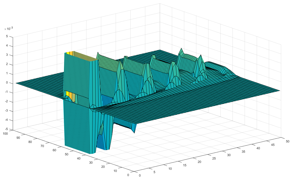
In this scenario, the pressure of a central element of a 50x50x50 cube simulation area is varied sinusoidally corresponding to a 8162 Hz wave. With reflecting walls, a sound vibration field is soon established. It is interesting to see the rapid drop-off in pressure from a point source as opposed to the relatively consistent pressure transmission once the wave spreads an appreciable amount. This is because the point source radiates in all directions (positive and negative x, y, z) while the later wavefronts only radiate in their propagation direction. The image below illustrates a slice through the center with the height corresponding to pressure level within the XY plane. The simulation is 3D, so a plot like the one shown exists at each of the 50 Z levels.
Evolution of pressure distribution with a point pressure sound source in a 50x50x50 grid (side length of 10cm). Slice along XY plane.
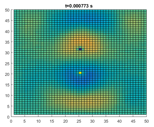
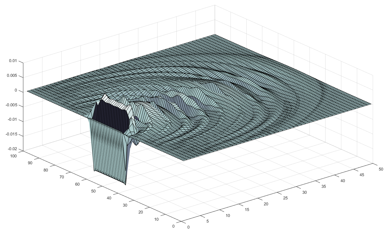
Instead of a sinusoidally varying pressure as above, what happens if the air velocity is varied sinusoidally? This is more representative of a speaker diaphragm moving back and forth, transferring its velocity to the air. It is seen that with this setup, both a high pressure and a low pressure area are formed at either end of the velocity segment. Thus the total pressure of the system is constant, a more realistic scenario than earlier.
Evolution of pressure distribution with a 2 cm long velocity (v_x) sound source in a 50x50x50 grid with side length of 10cm. Slice along XY plane.
Since both high and low pressure areas are produced next to each other, the propagation to either side of the velocity source becomes significantly attenuated due to destructive interference between the two areas. This looks similar to the action of a dipole radiator in the electromagnetic field. For a loudspeaker, better performance can be achieved by covering up one end of this dipole, making the device act as a pressure source and thus avoiding the destructive interference. This is why speakers are placed in airtight cabinets rather than just set bare (the sound reflections inside the cabinet might also help amplify low frequencies but are out of phase so usually directed backwards or to the side with a special opening in the cabinet - high end speakers are totally enclosed to avoid the out of phase sound).
A top view of the final step of above simulation, more clearly showing the dipole sound pattern that is established.
So far the acoustic equation seems to make no claim about frequency dependence of propagation. The presence of the scalar, pressure, means that each point can act as a point source. The observed wave propagation is the summation of many point sources (Huygens' principle, which also seems to apply to electromagnetic waves - this may not be such a surprise if the formulation also involves a scalar quantity). It was implicit in the rough derivation of the acoustic equation that the sound velocity is constant, so different frequencies will propagate at the same speed, although a rigorous proof of this would certainly be worthwhile. Instead I would like to focus on the diffraction of sound. This can be simulated by a constant size pressure source which oscillates with a wavelength either equal to the source size or much less than the source size.
It is claimed by many sources (my physics teacher, online videos and texts on sound diffraction) that long wavelengths will diffract more than short wavelengths. The typical example is that bass notes tend to be heard earlier than the high frequency notes when approaching a concert event (or a marching band), because the bass notes are lower frequency and can thus diffract around corners and through openings, reaching the listener even outside a direct line of sight. Meanwhile high frequency notes travel in straight lines and thus don't reach the listener that is around a corner. Yet, there is no frequency dependence in the acoustic equation. Each point acts as a point source and that's it. Is there any validity to the above claims of 'increased diffraction' at low frequencies? I simulate a plane wave incident on a single slit, where the slit is constant but wavelength is changed from equaling the slit width to four times shorter. If the claim is true, the spread of the long wavelength wave should be noticeably greater than that of the shorter wavelength wave. (There may be a mistaken 'derivation' of the frequency dependence by using a few arbitrarily arranged point sources, which turns the slit into a diffraction grating whence the frequency dependence comes from the distance between point sources. Here I use 20 to 50 closely spaced point sources to avoid such an outcome)

Wave diffraction through a single slit when the wavelength = slit width.
Wave diffraction through a single slit when the wavelength = (1/4) * slit width.
The case of wavelength = slit width certainly shows diffraction. But so does the shorter wavelength case! In fact the two are effectively the same! Here is a closer look at the last step of the simulations.
A top view of the long wavelength diffraction case.
A top view of the short wavelength diffraction case.
An overlay of the long and short wavelength diffraction pressure fields.
This isn't too convincing. In the overlay image above, the short wavelength edges seem to extend just as far out radially as the long wavelength edges. Perhaps my wavelength is still too long to see a real 'directionality' for sound? I reduce the simulation area to be able to accurately simulate a wave that is ten times shorter wavelength than the slit width, while keeping the slit width constant for reference.
An overlay of the long (slit width) and short (slit width / 10) wavelength diffraction pressure fields.
Even with a wavelength that is ten times shorter than the slit width, the spread is not appreciably smaller than the spread of the low wavelength wave. To me, this is a welcome conclusion since it seems a bit arbitrary to claim that shorter wavelengths can be more directional when a scalar pressure controls propagation. Why does the idea of 'greater diffraction' of low wavelengths of sound persist? This likely has to do with what is being compared. In the above simulations, I compared the effects of a pressure source of constant amplitude (pressure maximum and minimum) and varying frequency. Such a source is not constant-power, the radiated power increases with frequency squared. If I compared equal power sources, the high frequency source would become much lower amplitude and thus the diffraction fringes would be dominated by the low frequency source. Another complication is the ear's frequency and amplitude dependent response. It is known that the ear's sensitivity to low frequencies is much below that to higher frequencies, so for low frequency instruments to be audible, they need to radiate relatively more power than their high frequency counterparts (part of the reason why the low-frequency instruments take more effort to play - and why battery-powered fire alarms use high pitch sound). A third factor is the noise background; typically high frequency sounds are present on the street from cars/people/wind while low frequency sounds are less common, making a diffracted low frequency sound easier to detect. Combining the above factors may indeed make the 'increased diffraction' of low frequencies an illusion rather than a rigorous claim. Indeed there were many times when I have heard the high frequency sounds of an approaching car well before the low frequency sounds became clear, even when standing around a corner, contrary to the increased diffraction hypothesis.
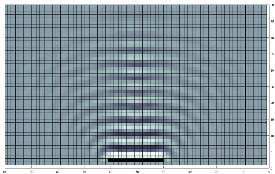
All of the above simulations used free-space pressure or velocity sources. In all cases, it was observed that a large decrease of sound amplitude resulted immediately after the source (which, in these cases was notably smaller than the wavelength). What happens if a tube is added around a point pressure source?
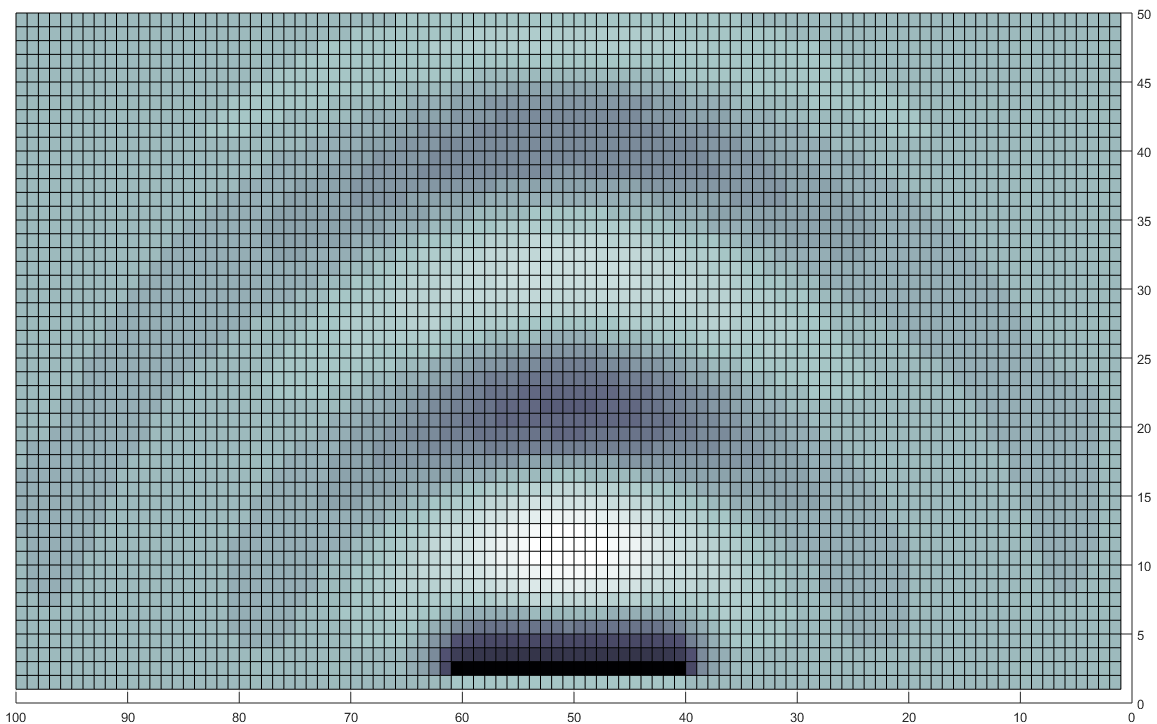
The 8162 Hz point pressure source from above is placed inside a reflective guide tube. The radiated pressure amplitude is noticeably higher than before.
Comparing to the point source simulation earlier, an improvement of about a factor of 2 in sound amplitude is achieved! This improvement comes since the high point pressure can equalize into a pressure wave inside the tube. The tube prevents a spread of the pressure wave in Y and Z directions, so the pressure source will tend to output more power. In the open case, pressure surrounding the point source quickly returns to zero, while in the covered case the point source remains surrounded by a higher pressure area because of the limited Y and Z propagation. Thus when the pressure source is driven low, there is a higher velocity established in the covered case. This view also supports the observed effect of wavelength and pressure source size - radiating a small wavelength from a small pressure source is much more effective than radiating a long wavelength from the same pressure source (already visible in the amplitude difference of the 10:1 slot width comparison overlay above). Keeping in mind that even the relatively high frequency 1 kHz has a wavelength of 31.4 cm, we now have a qualitative explanation for the use of spreading cones on concert loudspeakers, as well as for the effectiveness of passive devices like cone-shaped megaphones used by coaches/cheerleaders and plastic cones/reflectors that make cell phone speakers sound better (simply placing a cell phone inside a cup can make a quick sound improvement). It is not required to have a tube-like constraint around the sound source, a lesser improvement can be made even with a single wall reflector as long as it expands the effective size of the source before the wavefront's exposure to the free atmosphere.
This article showed that interpreting air as a collection of colliding molecules leads to the Maxwell-Boltzmann distribution and to a scalar (directionless) quantity (interpreted as pressure or as temperature) which can be established by a directional influence such as colliding molecules' velocity. Such a quantity made it possible to simulate large areas without tracking individual particles. From the simulation, point and dipole sources were observed, and tests of equal-amplitude single slit diffraction disproved the common quip that low frequency waves 'diffract more'. Loudspeakers behave as spherical sources of sound, whose efficiency in creating pressure waves may be improved by making the source as large as a wavelength of the sound, or by adding an expanding horn to do the same. The sounds heard when listening to a sound source in an open space consist of direct and reflected spherical wavefronts which, with only slight directional dependence (because of other objects in the space, and interference from multiple sound sources or slits), makes setting up a space for 'good acoustics' a relatively simple matter of adding sufficient absorption, diffusion, and reflection (by covering some walls, using carpet, and in extreme cases moving other objects like furniture).