There are many cases in which continuous quantities are recorded as symbols representing a finite signal width, for example in an electronic analog to digital converter (ADC) which outputs a bit value for a given voltage at a given time. In fact if we look more generally, anything we interact with is subject to these principles - we write down numbers with a finite number of digits, express ideas with a finite number of words, and experience reality as a finite number of sensations. If we assume that an underlying value exists at arbitrarily high precision, then there will be some rules describing how many measurements of a low precision are necessary to estimate that value. In the ADC case, taking multiple samples over time and averaging them is often used to obtain a less noisy value, but why does this work and what are the limitations?
In an ADC, an input voltage is compared to a reference voltage, and here I assume that noise on either of these voltages impacts the result in a similar way, so we may treat the system as an ideal (noiseless) ADC, a noiseless input signal, and a noise that intervenes in the measurement. In this manner, the three quantities may be represented as numbers with sufficient relative precision to simulate the situation where the ideal parts are unknown. The input signal, which is a real number, is discretized with the floor(x)+0.5 function which places numbers into "bins" whose edges are the integers. Thus each integer represents the threshold at which a change in the input signal causes a change in the least significant bit (LSB) of a digital output value.
The input signal is represented by a normal distribution with mean value rho and standard deviation sigma. To avoid the case of the signal being discretized into only one binary code when sigma is very low, I place the mean at a bit boundary, rho=0. Then even with low rho, we would expect a similar distribution of -0.5 and 0.5 discretized values which average out to zero. The case of different bit boundaries is considered towards the end of the discussion.
If we take some samples of the input signal, we would expect these samples to be normally distributed (since the signal is normally distributed). If we then average these samples, we get a mean of the sampled distribution. And if we repeat this process and plot the distribution of the means, we can obtain the standard deviation of the means. This is a metric of the precision we can expect for a mean of some number of samples. In the absence of discretization, it is clear that no averaging (or an average of 1 sample) will result in the same distribution as that of the signal. Increasing the number of samples in the average will not decrease the standard deviation of the input data batch, but it will decrease the standard deviation of the average value compared to the underlying "true" value. This is illustrated below.
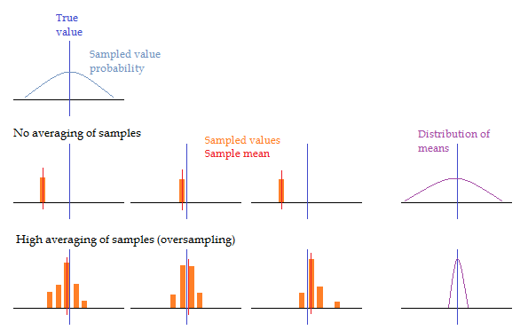
A visual illustration of the standard deviation of the means. Top left, on top of a horizontal number line, the vertical line represents a perfectly defined true value, and the curve represents the probability that a measurement result will be in the vicinity of the true value. In the following row, three individual random samples are shown on the number line, and if we continue to acquire samples in this manner we will recreate the input distribution. In the bottom row, three histograms of multiple random samples are shown. The mean value of these histograms (red vertical line) is distributed about the true value in a much tighter distribution than the input even when each histogram has a standard deviation matching the input.
I implemented this experiment numerically. 1000*N random values are generated, then discretized, then averaged together in groups of N. This gives 1000 averages, of which a standard deviation is calculated. This is repeated for different values of N as well as sigma of the input signal. The scilab code for this simulation may be downloaded here. This gives the following plot for sigma={1, 5, 10}.
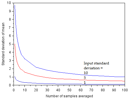
The horizontal axis represents N, the number of samples to average. The vertical axis represents the standard deviation of the average (closeness to true value). At the left edge, where N=1, the standard deviation of the sample is equal to the standard deviation of the noisy input. With more samples included in the average, the standard deviation is reduced.
As expected, the averaged value is closer to the true value as the number of samples in the average increases. The relation here is effectively indistinguishable from the 1/sqrt(N) reduction that is calculated in the continuous case. Therefore the discretization of the signal does not have a statistical impact even when the signal has sigma as low as 1 LSB. When will it have an impact?
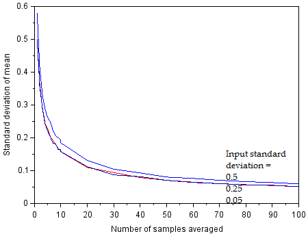
As the input sigma falls below 0.5 LSB, there is no longer an improvement in the averaged value. We are now limited by discretization noise.
The standard deviation is seen to reach a limit at sigma=0.5, where reducing sigma results in no improvement to the precision of the averaged value. This is the noise floor imposed by the discretization process, and it is visible because we have defined the distribution to be centered on a bit boundary. If the distribution were centered between two bit boundaries with very low sigma, the measured standard deviation would fall to 0, and we would have no way to quantify it. In fact, at such low noise levels we may get worse performance from the ADC! This comes from two factors. First, if the bit code never changes, we cannot use averaging to improve our actual standard deviation below 1 LSB even if this were otherwise possible. Second, if the true value is near a bit boundary, we may observe non-linearity in the transition between adjacent bits if the noise is not uniformly distributed (the normal distribution is not uniform, so the mean of a histogram of adjacent bit codes will not correspond to the true value). In a sense the two factors are the same thing (temporal distribution of noisy input not being spread nicely across multiple bit codes to allow averaging). This situation was simulated by shifting the center of the distribution from rho=0 to rho=1 while maintaining discretization boundaries at integer values, and evaluating the mean of means with N=100.
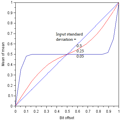
At low input sigma, the averaged value may not correspond to the true value due to the normal distribution either falling within one bit code, or due to the normal distribution causing a non-proportional spread of adjacent reported bit codes at a boundary.
It appears that as we reduce the noise level to zero, we lose the ability to gain any precision beyond 1 LSB through averaging (although we can expect to achieve this 1 LSB from just one sample). Could it be that noise is the secret ingredient to precision in discretized measurement? The simulation suggests that above sigma=0.5 the linearity between true value and average of samples is maintained, so there is no particular need for carefully shaped noise (such as a triangle wave which would be proportional in temporal distribution at bit boundaries) as long as this noise is sufficient to cover a few LSBs. At higher noise values, there is a loss due to the requirement for more samples to be included in the average to achieve a given precision as sigma/sqrt(N) LSB, which impacts the measurement bandwidth. At lower noise values, there is a loss of linearity and no effective improvement beyond 0.5/sqrt(N) LSB. Therefore an ideal noise value is in the range of sigma=(0.5 to 1) LSB. For reference the histograms of the bit codes for these distributions are shown below for the true value at bit boundaries (rho=0) and between bit boundaries (rho=0.5).
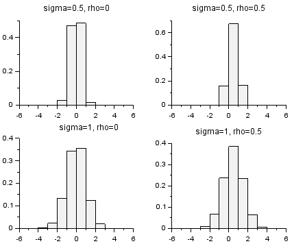
Histograms of discretized values of normal distribution with discretization boundaries at the integer values. The top vs bottom rows compare a change in sigma; the left vs right columns compare a change in rho. The vertical axis is probability distribution, and the horizontal axis is bit boundaries (LSB shifted by 0.5). Distributions narrower than the top plots, and distributions wider than the bottom plots, deviate further from optimal performance.
In designing an ADC data acquisition system, the above findings may be applied as follows. After setting up the system in a condition where the ADC will read a constant input value, acquire a large number of measurements (~1000) and plot them on a histogram with bins centered on each bit code. If you have a really clean signal path (or a coarse ADC) with the histogram narrower than the plots above, and resolution beyond 1 LSB is desired, consider adding noise to reach a width like the above; in the absence of added noise, the further described statistical calculations on the data may not be accurate. If the histogram does not look like a normal distribution, there may be noise sources which will not cancel out in the expected manner (such as noise synchronous with the conversion rate) so the calculations will be inexact. Calculate the standard deviation of the histogram, which may be taken as the standard deviation of the input signal in LSB (rho=sum(data)/length(data); sigma=sqrt(sum((data-rho).^2)/(length(data)-1))). Determine your desired resolution in LSB, and find the required number of averages by squaring the ratio between observed and desired sigma. The following table includes some calculated values for sigma to give an intuition of the requirements; sigma = 0.5 may be interpreted as +-1 LSB on the measurement result.
Desired sigma | 8 | 4 | 2 | 1 | 0.5 | 0.25 | 0.125 |
|---|---|---|---|---|---|---|---|
Observed sigma | N= | ||||||
| 8 | 1 | 4 | 16 | 64 | 256 | 1024 | 4096 |
| 4 | 1 | 4 | 16 | 64 | 256 | 1024 | |
| 2 | 1 | 4 | 16 | 64 | 256 | ||
| 1 | 1 | 4 | 16 | 64 | |||
| 0.5 | 1 | Uncertain | |||||
ADC hardware is often configurable for different sampling and conversion times, which affects the sample rate as well as noise level. In an ideal description, a longer hardware sampling time would have a similar impact as software averaging but without the computational overhead; in reality this is not necessarily true because noise sources within the ADC do not decrease at longer sampling times and the number of bits converted does not increase. There is no general rule, because of variations in noise type and magnitude, as well as hardware and software resources available for filtering. I would recommend plotting a histogram as described above for each hardware configuration of interest, and then comparing the results in terms of data rate and resolution taking into account any required averaging.
When implementing averaging of N samples, the measurement bandwidth will be reduced accordingly, from the nominal ADC sample rate SR, to SR/N. What about other impacts like a moving average filter or sampling at longer intervals (subsampling) but taking high frequency averages for each sampling instance? This is a discretization of the signal in time rather than in value. While not really a linear function (it may be seen as a sum of step functions multiplied with the input signal), it is possible to interpret the impact of discrete time sampling as a transfer function with a sinusoidal input and output. By simulating this numerically (scilab code), and taking FFTs of the input and output signal in various conditions, it is confirmed that this filtering does not generate harmonics, although the output Nyquist frequency may be lower than SR/2. So we may plot the change in magnitude and phase to observe the general impact of temporal discretization.
The transfer function of the moving average filter is computed. In this filter, data is sampled at rate SR, then N adjacent samples are averaged, then the averaging window is shifted forward by 1 sample; the output data rate is also SR. The resolution improvement on a static value due to averaging follows the rules described above while the transfer function shows the impact on bandwidth and phase. In the following calculation, SR=1000, N is varied, and the frequency of the signal is simulated from 0 to SR/2.
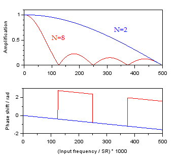
Amplification and phase shift of the moving average filter for N={2,8}.
The amplification of the moving average filter in the simulation matches the mathematical derivation [stackexchange ref1, ref2]. At higher values of N the response is of a similar nature, with zeros in gain at multiples of SR/N. We may roughly define a -3 dB point (gain of 1/sqrt(2)=0.7071) at Fc=SR/(N*2.25); a gain of 0.99 occurs at approximately Fp=SR/(N*12.2) and a gain of 0.999 occurs at approximately Fp=SR/(N*32.1). Interestingly, within the low-frequency region before the first zero in amplification (at SR/N) the phase shift is independent of Fc. At frequencies above SR/N the phase flips alternately at each subsequent multiple of SR/N with an overall downward trend. The moving average is not really a low-pass filter, because the gain has substantial peaks between multiples of SR/N and the roll-off is weak by filter standards. This suggests that the moving average should be used only when the signal frequency is well separated from noise frequencies, and when the noise is not substantial. Other filters before or after the moving average should be used to attenuate noise.
Another type of data processing would average N samples as above, but move forward between averages by M samples rather than by 1 sample. The output data rate is SR/M. This is the case of a system that acquires N samples at SR and averages them to produce a datapoint, then waits a relatively long time before acquiring another set of N samples. This is readily applicable when the input signal is slowly varying and oversampling is used to improve bit code resolution. In the case of M=N, the system acquires samples continuously at SR and averages each batch of N samples independently rather than with a moving window. We may simulate the transfer function with a few values of M.
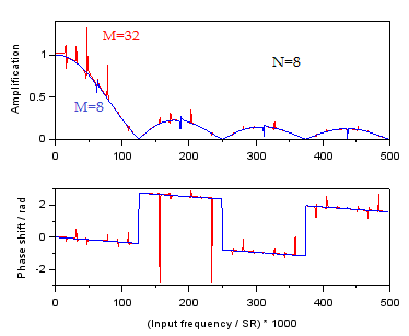
Amplification and phase shift of the block average filter for N=8, M={8,32}.
Effectively, a higher M introduces aliasing into the output stream. The gain and phase do not "behave nicely" near multiples of SR/(M*2) - note the factor of 2 due to the reduction on top of the Nyquist frequency. Keeping the signal bandwidth below SR/(M*3) will ensure minimal change in averaged value (0.001 x) and phase compared to the static case. One concern here is that the gain is above 1 near multiples of SR/(M*2), which means noise frequencies may be amplified in the output, and due to the reduction of output rate by 1/M it is no longer possible to filter out this noise. This is because SR is sufficient to capture the noise, and this is folded onto SR/M output stream in a frequency that cannot be resolved as different. Therefore, when using SR above the signal bandwidth (oversampling) while also not sampling continuously (undersampling), it would be prudent to include a hardware filter before the ADC which will eliminate frequencies above the signal bandwidth. Note this effect may be reduced by acquiring data with a jitter in the start of averaging (varying M over time) which would spread the amplified portions across the spectrum.
Based on the above, a set of guidelines may be stated for measuring a signal with ADC. For resolution of 1 part in 100, Fd=SR/(M*2.2) and Fc=SR/(N*12.2). For resolution of 1 part in 1000, Fd=SR/(M*3) and Fc=SR/(N*32.1). The highest frequency of interest in the signal should be below the lower of {Fd,Fc}. A hardware low-pass filter should be included that passes frequencies up to the higher of {Fd,Fc}. Using the histogram for a static ADC reading at a defined SR, N should be chosen to give a dynamic range matching the desired resolution with the expected signal amplitude.